Stochastic programming

7. Stochastic programming#

7.1. Addressing parametric uncertainty#

We can distinguish two broad kinds of uncertainty (recall the discussion of uncertainty in Section 3): structural uncertainty and parametric uncertainty. Structural uncertainty pertains to uncertainty in the model’s structure: we are not certain if the model is an appropriate representation of reality. For example, it could be oversimplified in a way that limits its usefulness for our intended application because we model nonlinear relations with linear equations. Parametric uncertainty stems from limited information on the parameters in the model: the numbers we feed into it. Assuming the structure of our model is broadly fine, we may still be uncertain about the exact value of particular parameters to fill in, such as electricity demand or wind power generation. We will only discuss this second type of uncertainty here.

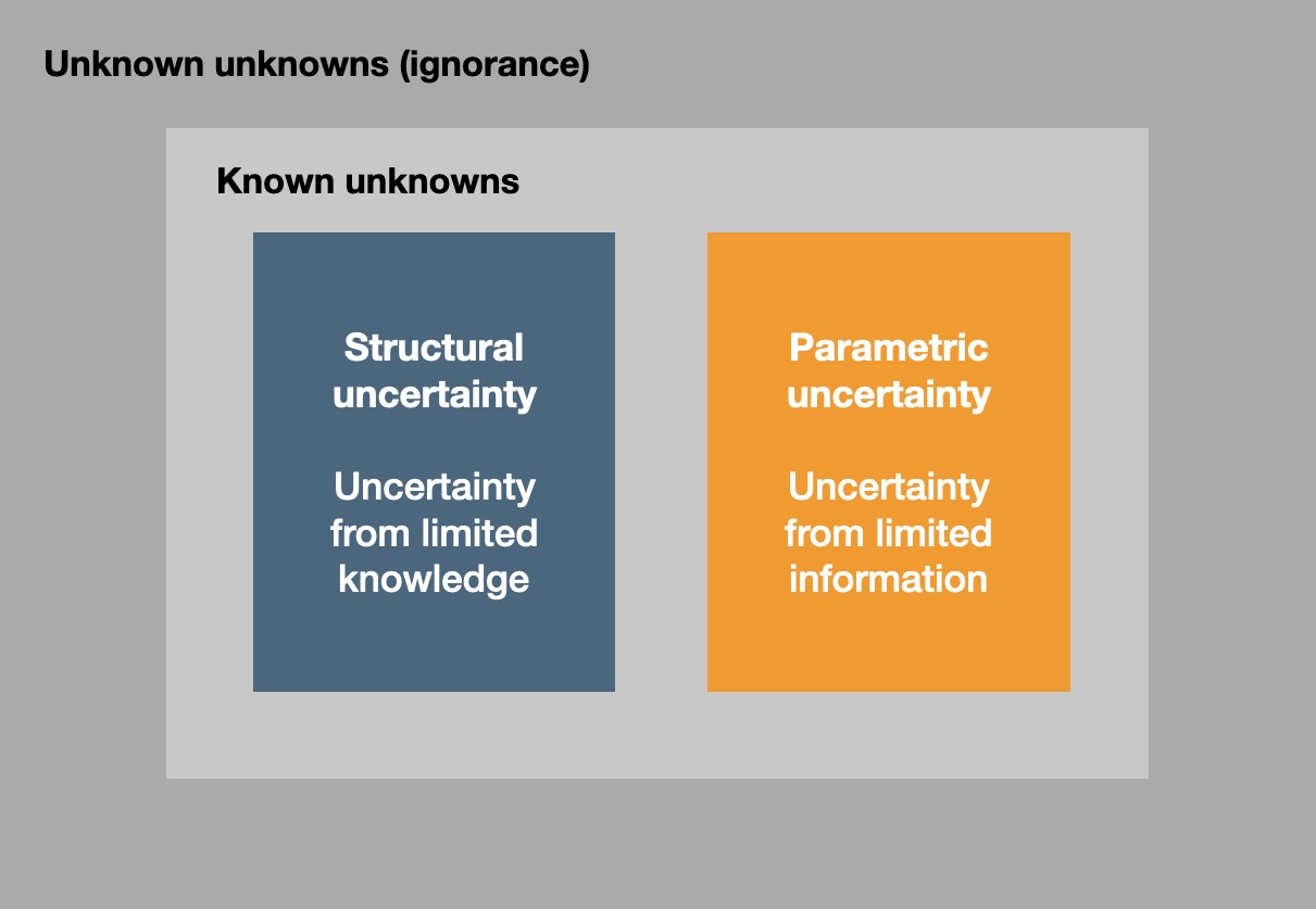
../_images/uncertainty-types.jpg — Fig. 7.1 Parametric uncertainty in the context of broader uncertainty. Based on a talk by David Spiegelhalter, “Uncertainty in Decision Models” (not available online).#

We have already covered sensitivity analysis in Section 3. We checked how the optimal solution changes as parameters in the problem formulation change. An alterative to sensitivity analysis is robustness analysis: here, we take a solution (e.g. the optimal solution) and investigate how well it performs when parameters change. Like sensitivity analysis, this is done after the model is solved. You can read more about robustness analysis in [Starreveld et al., 2024].

What about methods that allow us to incorporate uncertainty already when we formulate a model? There are two widely-used approaches for doing that.

First, there is stochastic programming. In stochastic programming, we explicitly model the fact that some parameters are uncertain, and we assume that we know the probabilities of specific outcomes for these parameters. We can set up several scenarios with known probabilities and formulate our problem such that all scenarios are considered, along with their probabilities, in solving the optimisation problem. As a result, stochastic programming can tell us what decisions to make based on our uncertainty quantification in the form of scenarios and their probabilities. Its usefulness depends heavily on how well these scenarios represent the uncertainties they represent.

Second, there is robust optimisation. Here also, we explicitly model the fact that some parameters are uncertain. There are different kinds of robust optimisation, but most commonly, problems are formulated so that the worst-case realisation of uncertain parameters is accounted for (and thus optimised for). At the same time, robust optimisation ensures that the solution is feasible for all possible realisations of the uncertain parameters. So we have a solution that is guaranteed to work, based on our assessment of the uncertainty in parameters, and works best in their worst-case realisation.

Robust optimisation is very different from how stochastic programming deals with uncertainty: rather than optimising for a single (worst-case) outcome, stochastic programming allows us to explicitly consider different uncertain outcomes—if we can describe these uncertain outcomes as a set of scenarios with given probabilities (which, in practice, can be difficult or even impossible).

The following table gives a high-level overview of some methods to deal with parametric uncertainty:

Table 7.1 Overview of parametric uncertainty methods#
	Stochastic programming	Robust optimisation	Sensitivity analysis	Robustness analysis
When to do it	When formulating the model	When formulating the model	After we solve the model	After we solve the model
What you need	Explicit quantification of scenarios with their probability for uncertain variables	Specification of an uncertainty set for uncertain variables	Access to shadow prices, or a set of scenarios for parameter values to test	A model solution to test under different scenarios
What you get	Solution that includes the possibility for recourse—choosing one of several alternatives once we know more about the realisation of uncertain parameters	Solution that is feasible for any possible realisation of the uncertain parameters, and optimal for the worst case	Effect of changes in limited numbers of parameters on the optimal solution (e.g. by looking at shadow prices), but only for small perturbations around the optimal solution	Effect of changes in limited numbers of parameters on the feasibility of a fixed solution, but only for small perturbations in parameters
Where to read more	Below in this chapter	In a future version of this reader	Section 3	[Starreveld et al., 2024]

For the remainder of this chapter, we will focus on stochastic programming.

7.2. Using scenarios to characterise uncertainty#

In stochastic programming, we deal with uncertainty by considering scenarios for uncertain parameters. This means we have discrete forecasts of the future that we can assign probabilities of occurence to (see Fig. 7.2).

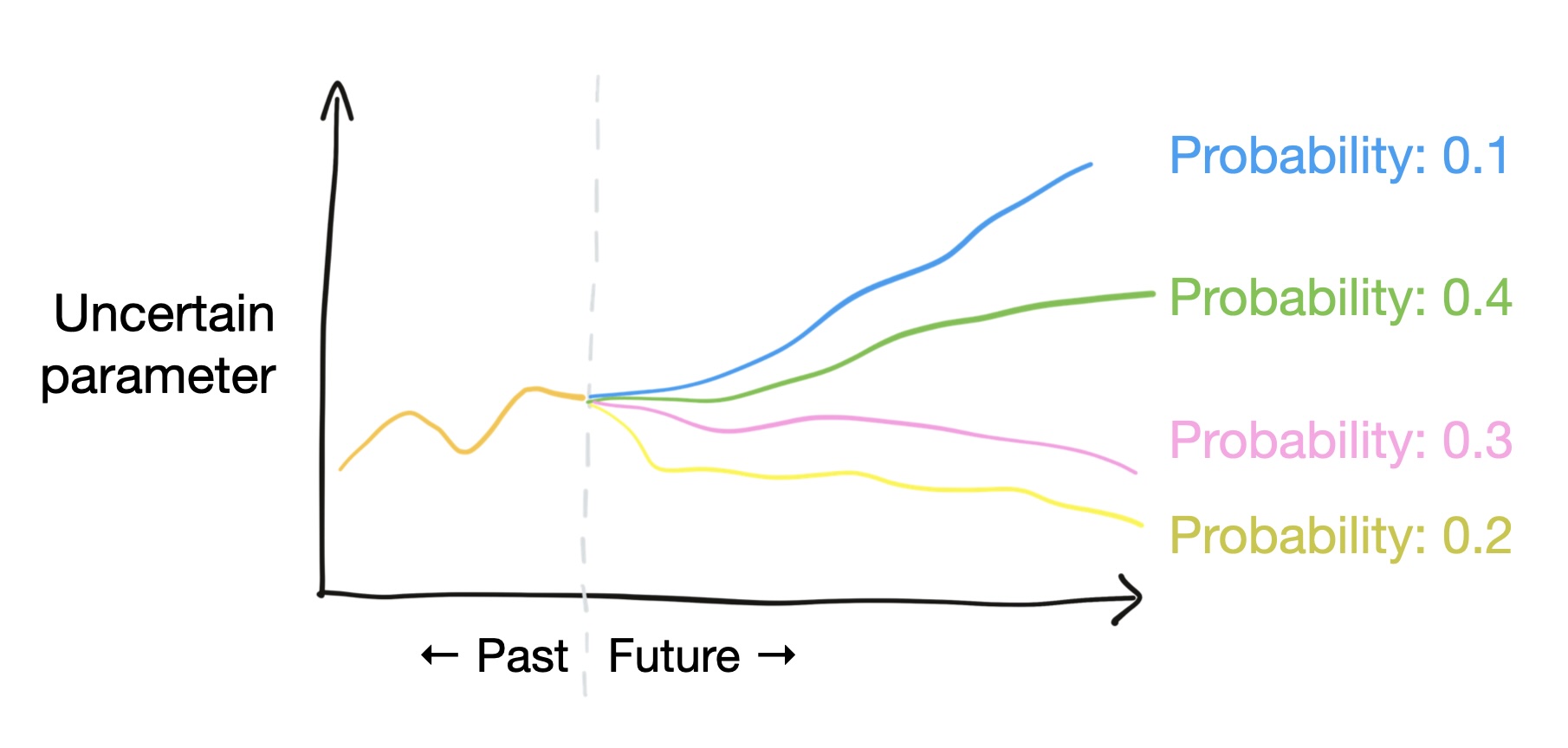
../_images/stochastic-scenarios.jpg — Fig. 7.2 In stochastic programming, uncertainty is represented as scenarios for the uncertain parameters with probabilities of occurrence.#

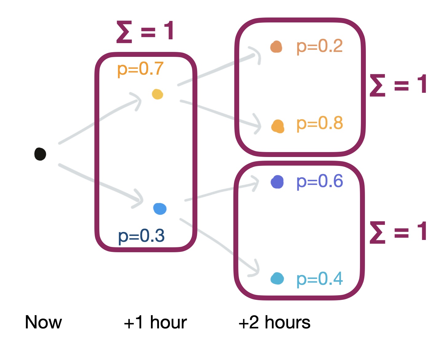
How can we construct such scenarios? Since we are considering discrete steps of time, $t = 1$ , $t = 2$ , and so on, we can build a scenario tree. Fig. 7.3 shows such a scenario tree for uncertain power prices over the next two hours. The prices are represented as a stochastic process leading to four scenarios. A stochastic process is a probability distribution over a set of paths describing the expected evolution of a random or uncertain variable. Each scenario is one realisation of the stochastic process.

../_images/stochastic-scenario-process.jpg — Fig. 7.3 Uncertain power prices over the next two hours can be represented as a stochastic process in four scenarios.#

We can combine the branches in the different scenarios and list them in a table. The probability of each scenario is calculated as the probability of one time step multiplied by the probability of the next step. The probabilities of all the scenarios need to sum to one. The power prices in each scenario in this example are also shown in Table 7.2 below.

Table 7.2 Scenarios#
Scenario	Power price in 1 hour	Power price in 2 hours	Probability
1	54	56	0.7*0.2=0.14
2	54	52	0.7*0.8=0.56
3	46	48	0.3*0.6=0.18
4	46	44	0.3*0.4=0.12

The next step is to actually integrate discrete scenarios like the ones above, for which we know probabilities, into our optimisation problem, turning it into a stochastic optimisation problem.

7.3. Stochastic programming for a demand response problem#

For this, let’s turn to a new example. In this example, we want to adjust electricity demand to match the fluctuating supply of renewable electricity sources (and therefore, the fluctuating electricity cost). Let us assume that a consumer performs a certain task that requires the use of electricity. This consumer’s utility function $f_{t} (u_{t})$ measures the benefit of consuming electricity $u_{t}$ for the task during time period $t = 1, . . ., T$ .

We will consider four time periods ( $T = 4$ ). For simplicity, we’ll assume that the marginal benefit is the same for each time period (it is independent of $t$ ) and $f_{t} (u_{t})$ is a linear function of electricity consumption $u_{t}$ . In other words, $f_{t} (u_{t}) = b \cdot u_{t}$ . Assuming the marginal benefit is constant over time means the task can be performed at any time, i.e. the electricity demand is deferrable.

There are, however, some limits on electricity consumption. For each time period $t$ , the consumption cannot be higher than 3 kWh. This is, for example, because the customer’s connection to the grid has a maximum capacity of 3 kW. Furthermore, the total consumption in the four time periods together must be between 6 and 8 kWh: the consumer requires at least 6 kWh but is willing to use as much as 8 kWh. Lastly, there are ramping limits (up and down) of 1.5 kWh between any two time periods: the machinery that demands this electricity cannot turn on or off instantaneously.

Our objective function is to minimise the difference between the cost of purchasing electricity and the benefit brought about by consuming such electricity.

7.3.1. 0 Parameters#

We know that the total consumption for the four time periods together must be between 6 and 8 kWh.

We also know the consumption cannot be higher than $U_{m a x}$ = 3 kWh for each time period $t$ .

We also know the ramping limit (up or down) is $U_{r a m p}$ = 1.5 kWh between any two time periods.

We will use the parameter $b$ = 100 €/kWh in the linear utility function. So, $f_{t} (u_{t}) = 100 u_{t}$ .

Now we introduce uncertainty with a stochastic process. Electricity price $λ$ per time period is an uncertain parameter. We consider price uncertainty with scenarios, indexed by $ω$ . $λ$ is the set of possible realisations of the stochastic process, or prices. $λ_{ω}$ is a vector representing one possible realisation of the stochastic process. Each realisation $λ_{ω}$ is associated with a probability $π_{ω}$ . In this example, we consider two scenarios with the probabilities $π_{1}$ and $π_{2}$ , which add up to 1. The table below shows the scenarios we consider.

Scenario	Probability	Price	Price	Price	Price
$ω$	$π_{ω}$	$λ_{1}$	$λ_{2 ω}$	$λ_{3 ω}$	$λ_{4 ω}$
1	0.5	120	105	154	84
2	0.5	120	45	66	36

So, we have two scenarios with 50% probability each. We can see that $ω_{1}$ is a high-price scenario and $ω_{2}$ is a low-price scenario. Also, we consider that the price is certain in period 1 and uncertain afterward. Therefore, $λ_{1} = 120$ in both scenarios. Then, there are two paths (the scenarios) for how the price could evolve in time. Periods 2, 3, and 4 are the uncertain part.

7.3.2. 1 Variables#

We want to decide how much electricity to consume $u_{t ω}$ during time period $t = 1, . . ., T$ . Because we have two scenarios, and one certain time period, there are seven optimisation variables: $u_{1}, u_{21}, u_{31}, u_{41}, u_{22}, u_{32}, u_{42}$ (the consumption at $t = 1$ and the scenario-dependent consumption at $t = 2, 3, 4$ ).

In other words, and this is the first key aspect of stochastic programming, we simultaneously consider (and make decisions about) several alternative futures (=scenarios). For each of these futures, we have a full set of decision variables, i.e. for scenario 1: $u_{21}, u_{31}, u_{41}$ .

7.3.3. 2 Objective#

Our objective is to maximise welfare (minimise costs minus benefits):

(7.1)#

min λ_{1} u_{1} - f_{1} (u_{1}) + \sum_{ω = 1}^{Ω = 2} π_{ω} \times \sum_{t = 2}^{T = 4} (λ_{t ω} u_{t ω} - f_{t} (u_{t ω}))

The objective function consists of three parts, and this is the second key aspect of stochastic programming:

The certain part, where $t = 1$ , in blue.
In orange, the summing up of each uncertain scenario weighted (multiplied) by its probability.
The uncertain part, where $t > 1$ , in green. For each scenario, we sum up over all timesteps inside the scenario (from $t = 2$ through $t = 4$ ).

7.3.4. 3 Constraints#

We have three practical constraints to consider.

First, the consumption per time period cannot be higher than $U_{m a x}$ = 3 kWh:

(7.2)#

U_{m i n} \leq u_{t} \leq U_{m a x}

Second, the total consumption for the four periods together must be between 6 and 8 kWh.

Third, there is a ramping limit of 1.5 kWh between time periods.

7.3.5. Full problem#

In our example, we end up with the following optimisation problem:

Variables: $u_{1}, u_{21}, u_{31}, u_{41}, u_{22}, u_{32}, u_{42}$
Objective (to be minimised):

(7.3)#

\begin{aligned} J = & (120 - 100) u_{1} + 0.5 [(105 - 100) u_{21} + (154 - 100) u_{31} + (84 - 100) u_{41}] \\ + 0.5 [(45 - 100) u_{22} + (66 - 100) u_{32} + (36 - 100) u_{42}] \end{aligned}

Consumption per time period constraint:

(7.4)#

\begin{aligned} 0 \leq u_{1} \leq 3 \\ 0 \leq u_{t ω} \leq 3 & ω = 1, 2, t = 2, 3, 4 \end{aligned}

Total consumption constraint:

(7.5)#

\begin{aligned} u_{1} + \sum_{t} u_{t ω} \leq 8 & ω = 1, 2, t = 2, 3, 4 \\ u_{1} + \sum_{t} u_{t ω} \geq 6 & ω = 1, 2, t = 2, 3, 4 \end{aligned}

Ramping limits constraint:

(7.6)#

\begin{aligned} u_{1} - u_{0} \leq 1.5 & ω = 1, 2, u_{0} = 0 \\ u_{2 ω} - u_{1} \leq 1.5 & ω = 1, 2 \\ u_{t ω} - u_{(t - 1) ω} \leq 1.5 & ω = 1, 2, t = 3, 4 \\ u_{0} - u_{1} \leq 1.5 & ω = 1, 2, u_{0} = 0 \\ u_{1} - u_{2 ω} \leq 1.5 & ω = 1, 2 \\ u_{(t - 1) ω} - u_{t ω} \leq 1.5 & ω = 1, 2, t = 3, 4 \end{aligned}

7.3.6. Optimal solution#

This is a simple linear optimisation problem (LP) that we can solve with the usual methods, e.g. by formulating and solving it with a mathematical programming language and solver.

The optimal solution is:

Scenario	$u_{1}$	$u_{2 ω}$	$u_{3 ω}$	$u_{4 ω}$	Total $u$
1	0.25	1.75	1.25	2.75	6
2	0.25	1.75	3	3	8

Notice that the total consumption is exactly at the limit in both scenarios. In the scenario with high prices (scenario 1), we consume as little as possible, at the minimum limit. In the scenario with low prices (scenario 2), we consume the maximum possible. This shows how important the total consumption constraint is in this example – it is always binding.

7.3.7. Interpreting the optimal solution#

What we have formulated and solved here is a two-stage stochastic programming problem.

In the first stage (“here and now”, $t = 1$ ), there is no uncertainty, so we make decisions $u$ , which do not depend on the realisation of the uncertain parameters. The uncertain parameters (price in our example) in the first time period $t = 1$ are certain so we can decide how much electricity to consume now, $u_{1}$ .

Then, time ticks forward by one time step; we arrive at $t = 2$ , in the second stage (“wait and see”). At this point the outcome $λ_{ω}$ of the uncertain parameter $λ$ is realised: we can observe whether we have ended up in the high price scenario or the low price one. Depending on which scenario we end up in (or in reality, perhaps, depending on which scenario we are closest to), we now follow either the decisions given by $u_{t 1}$ or by $u_{t 2}$ .

In summary, the sequence of events is thus:

First stage (here and now): the decision $u_{1}$ not depending on the realisation of the uncertain parameter is made.
The outcome $λ_{ω}$ of the random parameter vector $λ$ is realised.
Second stage (wait and see): decisions $u_{t ω}$ are made according to $λ_{ω}$ .

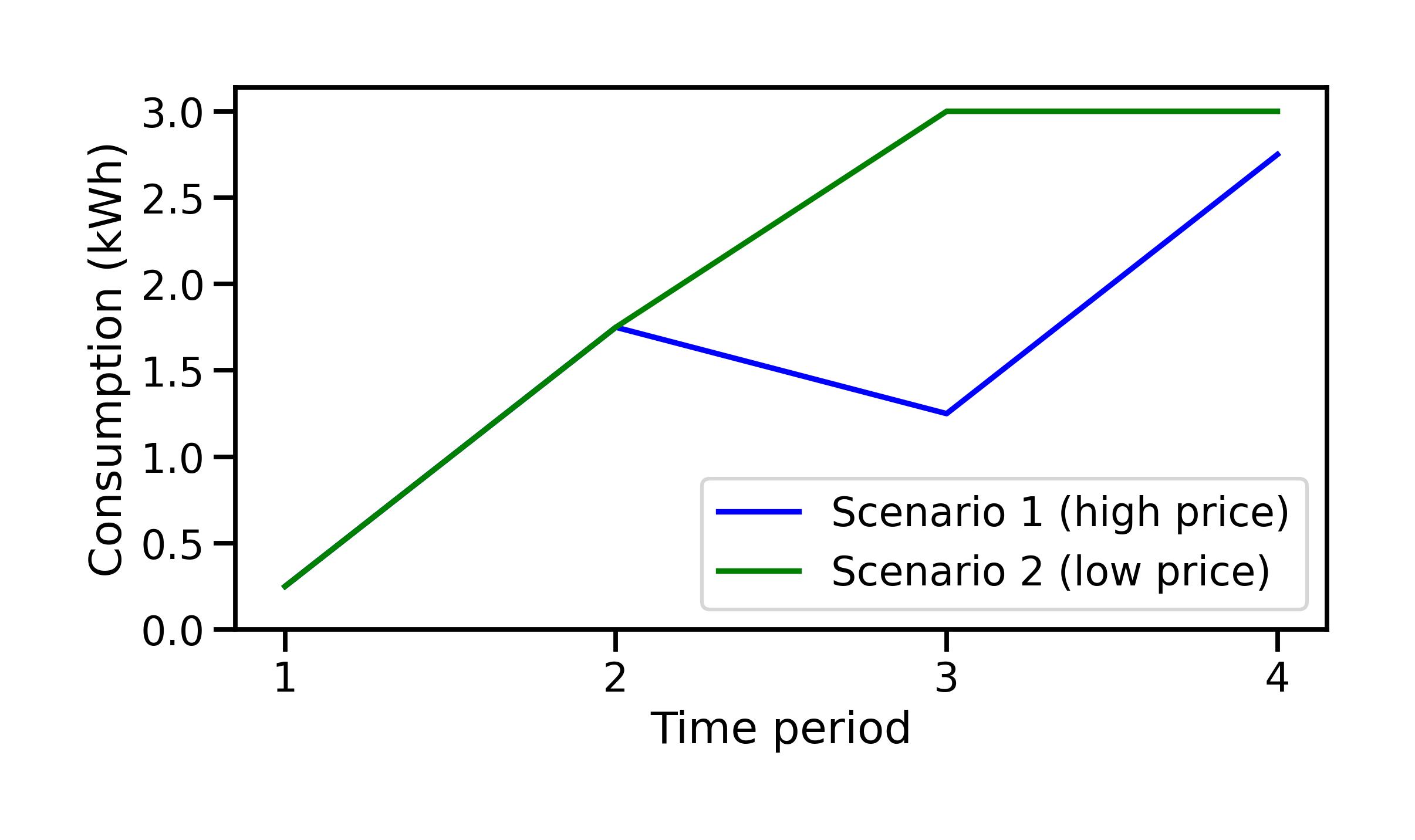
../_images/fig_stochastic.jpg — Fig. 7.4 Optimal solution for electricity consumption during each time period, for the two scenarios.#

What is crucially important to realise is that we have incorporated the uncertainty described by the scenarios into our problem formulation and thus into our decisions. Though we know with certainty what the price is in $t = 1$ , the formulation of including both the certain and uncertain part in the objective function implies that even the decision at $t = 1$ is influenced by the uncertainty that follows. We can say that the decision taken here and now is chosen so that it is optimal for either of the two possible follow-up scenarios.

Multi-stage stochastic problems

Here we have formulated and solved a two-stage stochastic problem. In principle we could consider $> 2$ stages and turn this into a multi-stage problem. However, problem size explodes dramatically with every stage that we add and quickly becomes computationally infeasible. So, as often, there is trade-off here between model “realism” and computational limitations.

7.3.8. Comparison to a case without uncertainty#

Let’s compare this result with a solution that considers no uncertainty at all. A reasonable way to do so would be to construct a “central estimate” between the high and low price scenario:

Scenario	Probability	Price	Price	Price	Price
$ω$	$π_{ω}$	$λ_{1}$	$λ_{2 ω}$	$λ_{3 ω}$	$λ_{4 ω}$
1	0.5	120	105	154	84
2	0.5	120	45	66	36
no uncertainty	1	120	75	110	60

We need to adjust our problem formulation to solve this simple LP problem. The objective function becomes:

(7.7)#

J = (120 - 100) u_{1} + (75 - 100) u_{2} + (110 - 100) u_{3} + (60 - 100) u_{4}

We only have the four decision variables $u_{1}$ through $u_{4}$ since we have no scenarios to consider. The constraints are simplified accordingly. If we solve this problem, this is the solution we obtain (compared to the two scenarios from the stochastic formulation):

Table 7.3 Comparison between stochastic and non-stochastic solutions.#
Scenario	$u_{1}$	$u_{2 ω}$	$u_{3 ω}$	$u_{4 ω}$	Total $u$
1	0.25	1.75	1.25	2.75	6
2	0.25	1.75	3	3	8
no uncertainty	1	2.5	1.5	3	8

What is happening here? The first observation is that the decisions taken without consideration of uncertainty are completely different from those taken in the stochastic formulation, already from the first hour $t = 1$ .

The decisions taken without consideration of uncertainty are more “bold” or “risky”: we “know” with certainty (at least our problem is set up that way) what the price will be in all four hours. We therefore know that we will be making a profit in hours 2 and 4 when the price is low, and we will already “get in position” in hour 1 to ramp up to a higher demand in hour 2.

The decisions taken in the stochastic formulation are more cautious at the start, with a smaller demand at $t = 1$ , in order to be able to react to either high or low prices later: if the price rises, it is best to limit consumption (to 6) while maximising it in the last time period with the lowest price. In contrast, if the price falls later, consumption can ramp up through $t = 2$ and $t = 3$ . The decision for $t = 1$ accounts for both of these possibilities. Note also that the ramping limits influence all these decisions: we cannot go from 0 to 3 and back to 0 to consume only in the more beneficial hours.

Fig. 7.5 shows an overview of the decisions taken in both the stochastic formulation and the formulation without uncertainty.

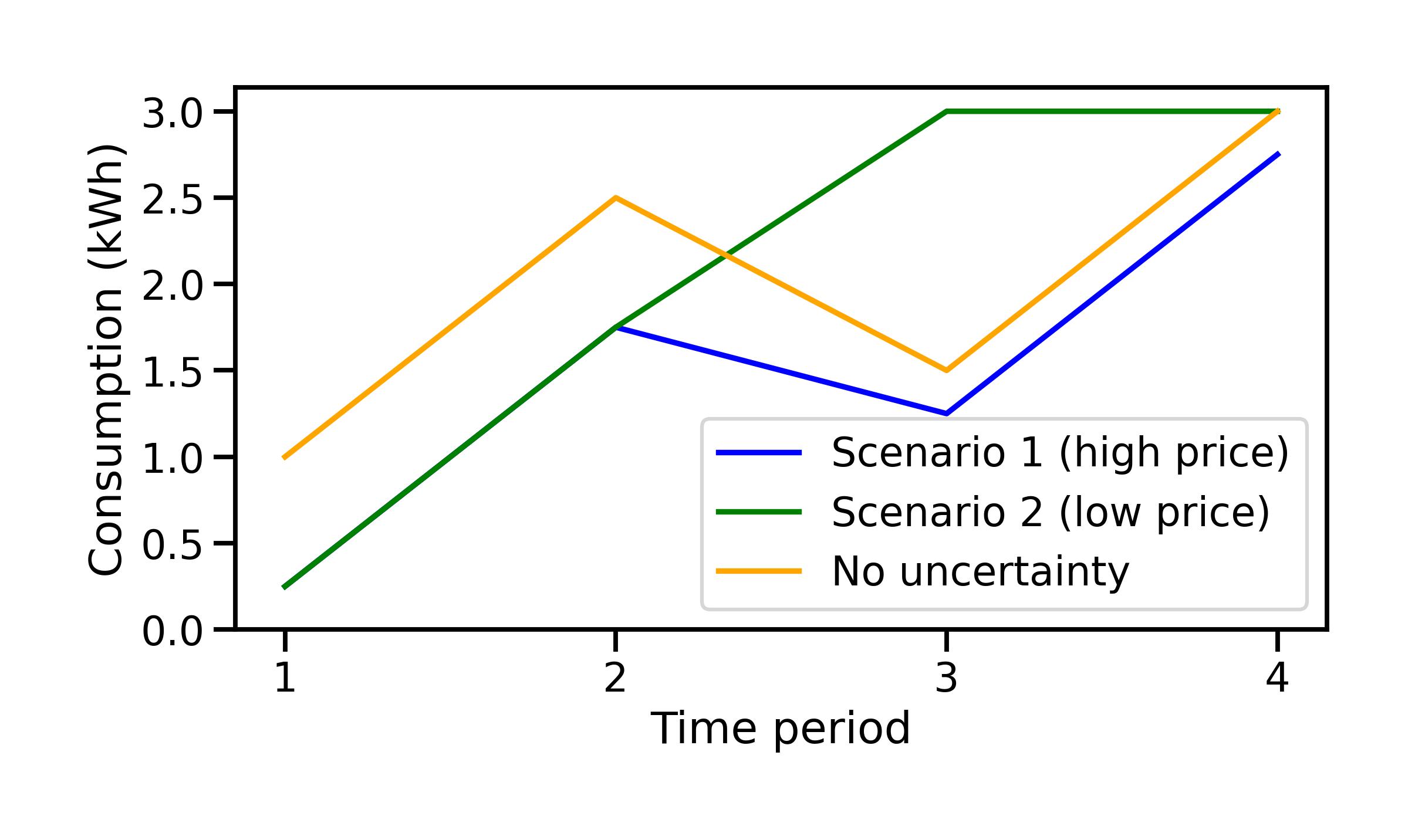
../_images/fig_stochastic_with_no_uncert.jpg — Fig. 7.5 Optimal solution for electricity consumption during each time period, for the two scenarios, and including the case without uncertainty.#

Finally, let’s look at the objective function values. Remember, we are minimising, so the smaller the value, the better. In the stochastic problem, the optimal objective function value is $- 174$ . This is made up of both decision branches in the uncertain part of the problem, so for it to be comparable to the formulation without uncertainty, we need to break it up into a part for just $u_{1}$ and $u_{t 1}$ , and another for $u_{1}$ and $u_{t 2}$ . So for the former, we take only the relevant decisions from the objective function and drop the multiplication with probability:

(7.8)#

(120 - 100) \cdot 0.25 + (105 - 100) \cdot 1.75 + (154 - 100) \cdot 1.25 + (84 - 100) \cdot 2.75 = 37.25

We end up with the following across all cases:

Stochastic problem ( $u_{t 1}$ , high price scenario): $37.25$
Stochastic problem ( $u_{t 2}$ , low price scenario): $- 385.25$
No uncertainty: $- 147.5$
No uncertainty (in the high price scenario): $65.5$

Note that the performance of the stochastic problem is better (=lower objective function value) than that of the case without uncertainty in the high price scenario. This last entry in the list comes from a small robustness analysis (see Table 7.1). We take a solution, in this instance the decisions from the case without uncertainty (bottom row in Table 7.3), and investigate how well it performs when parameters change, in this instance using the prices from scenario 1 (high prices).

(7.9)#

(120 - 100) \cdot 1 - (105 - 100) \cdot 2.5 + (154 - 100) \cdot 1.5 + (84 - 100) \cdot 3 = 65.5

Not surprisingly, if the prices are higher than expected in the case with no uncertainty, the modelled decisions do not perform so well. The objective function which we are trying to minimise is objectively worse than in the other cases.

7.4. References#

[SBD+24] (1,2)

Justin Starreveld, Gregor Brandt, Jaron Davelaar, Dick den Hertog, Zofia Lukszo, and Nort Thijssen. Robustness analysis for adaptive optimization with application to industrial decarbonization in the netherlands. ():, 2024.