5. Power markets and mixed-integer programming

Before we move on to modelling the day-ahead auction in the European electricity market, we will make some refinements to our unit commitment example from Section 2.1. In Section 5.1 we will allow power plants to shut down, and in Section 5.3 we will introduce a first constraint that connects the state of our system across different time periods. The first of these refinements will require us to introduce a new kind of variable: binary variables which can only take the value of either \(0\) or \(1\). As we will see, this makes problems computationally more difficult to solve, but is sometimes necessary to more accurately model a real-world situation.

5.1. Allowing power plants to turn off: from economic dispatch to unit commitment

We once again return to the economic dispatch problem from Section 2.1 (Fig. 5.1). We want to make one important addition to it: the ability for power plants to be turned on and off. In the original formulation, the \(\geq\) constraints on the plant power outputs prevent a plant from ever turning off. In order to allow a plant to turn off while still enforcing that it has some minimal power output if it is turned on, we need to introduce additional variables.

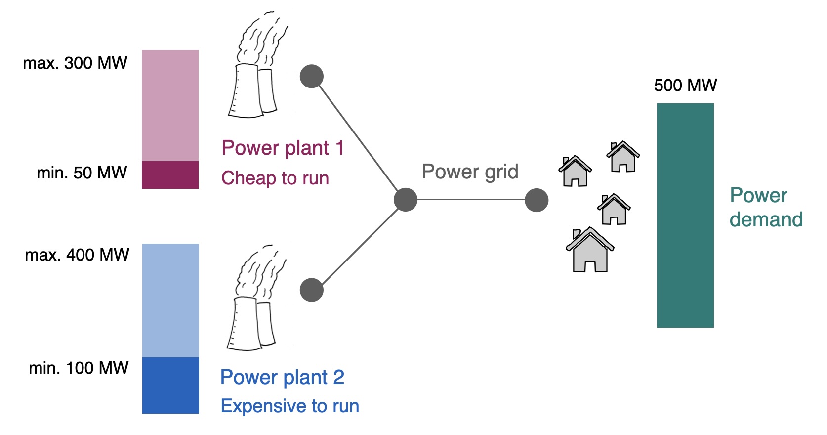
Fig. 5.1 Our economic dispatch problem with two power plants.

5.1.1. Additional 1 Variables

We want to decide how to operate our units, so we still have the power generated in each unit as variables: \(P_{Gi}\). We also want to decide whether a unit is on or off, and we can represent this with an additional set of variables: \(u_i\). \(u_i\) is a binary variable where 0 means the unit is off and 1 means the unit is on.

5.1.2. Additional 3 Constraints

We need to modify the constraints that enforce the minimum and maximum generation limits for each unit. We include the binary variables \(u_i\) as follows:

(5.1)\[\begin{equation} u_i P_{Gi}^{min} \leq P_{Gi} \leq u_i P_{Gi}^{max} \quad i = 1,...,n \end{equation}\]

This allows our model to “decide” whether a plant is on or off. Let’s say \(u_1\) is \(0\). Then the constraint for unit 1 becomes:

(5.2)\[\begin{equation} 0 P_{G1}^{min} \leq P_{G1} \leq 0 P_{G1}^{max} \end{equation}\]

Or rather:

(5.3)\[\begin{equation} 0 \leq P_{G1} \leq 0 \end{equation}\]

In other words, it allows (and even forces) \(P_{G1}\) to be zero. If \(u_1\) is \(1\), the min/max output constraints apply in the same way as they did in our original economic dispatch problem.

Importantly, this only works if the variable \(u_i\) is a binary variable:

(5.4)\[\begin{equation} u_{i} \in \{0, 1\} \quad \forall i \end{equation}\]

5.1.3. Full problem

Our objective remains to minimise the total cost of generating power. Besides the additions made above, the rest of our problem stays the same as in Section 2.1.

So our full unit commitment problem is the following:

• 1 Variables: Power output \(P_{G1}\), \(P_{G2}\), On/off state of each unit \(u_1\), \(u_2\)

• 2 Objective (total generation cost, to be minimised): \(C = 3 P_{G1} + 4 P_{G2}\)

• 3 Constraints:

  • Demand balance constraint: \(P_{G1} + P_{G2} = 500\)

  • Operational constraints for unit 1: \(u_1*50 \leq P_{G1} \leq u_1*300\)

  • Operational constraints for unit 2: \(u_2*100 \leq P_{G2} \leq u_2*400\)

  • Binary variable constraints: \(u_{i} \in \{0, 1\} \quad \forall i\)

To solve this problem, we need an approach to deal with the newly-introduced binary (integer) variables.

5.2. Mixed-integer linear programming (MILP)

If we add binary (0/1) or integer (…, -1, 0, 1, 2, …) variables to our problem, we turn it from an LP (linear programming) to MILP (mixed-integer linear programming) problem.

We consider a simple example (from Hillier and Lieberman [2021]). Consider this linear optimisation problem:

(5.5)\[\begin{align} \max &~ Z = x_1 + 5x_2 \\ \text{s.t.}&~ x_1 + 10x_2 \leq 20 \\ &~ x_1 \leq 2 \\ &~ x_1 \geq 0 \\ &~ x_2 \geq 0 \end{align}\]

We can contrast the above problem to this slightly modified version, where we introduce the additional constraint that \(x_1, x_2\) are integer variables:

(5.6)\[\begin{align} \max&~ Z = x_1 + 5x_2 \\ \text{s.t.}&~ x_1 + 10x_2 \leq 20 \\ &~ x_1 \leq 2 \\ &~ x_1 \geq 0 \\ &~ x_2 \geq 0 \\ &~ x_1, x_2 \text{ are integers} \end{align}\]

How do the optimal solutions to these two problems compare? Counter-intuitively, as we can see in Fig. 5.2, the optimal solution to the mixed-integer (MILP) problem is quite far away from the solution to the purely continuous (LP) problem: the red dot shows the optimal solution if \(x_1\) and \(x_2\) are continuous, the orange dot shows the optimal integer solution (note that the integer constraints turn the feasible region from the grey space to the set of blue dots). This example demonstrates that it is not straightforward to solve an MILP problem: we cannot simply solve an LP version of the problem and then look for the closest integer solution by “rounding” our variable values to integers.

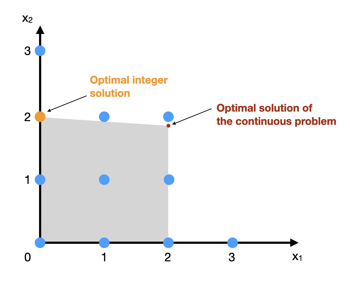
Fig. 5.2 Comparing a continuous LP to mixed-integer LP (based on Hillier and Lieberman [2021] Figure 12.2)

5.2.1. Branch-and-bound approach to solving MILP problems

The branch-and-bound method is one way to solve MILP problems. The idea is that we build a decision tree with each node of the tree being a MILP problem and each branch being a value of an integer or binary variable. The tree starts from the LP relaxation of the original problem—we solve the continuous problem first to give us starting values of the decision variables. Then we explore the branches—different combinations of the integer or binary variables. Since real-world problems involve many variables, it would take too much time to solve all the possible MILP problems, so we eliminate the branches that are not going to lead towards the optimal solution. This is the bounding part of the method. The idea is to fix one variable to an integer value at a time, while allowing the other variables to be continuous, then solving the problem to find upper/lower bounds of the objective function value. If a branch does not lead to a better upper/lower bound of the solution (or a feasible solution at all), then we cut off that branch and stop exploring that direction.

The details of this are outside our scope. But what is important to note is that solving an MILP problem involves solving a series of LP problems. This can increase the computational requirements to solve a problem quite dramatically.

5.3. Multi-period unit commitment: connecting what happens across time steps

Before moving to power markets, let’s make one final modification to the unit-commitment problem that we will later also carry across to the markets.

So far, we only considered a single isolated time period (for example, a single hour). Now, we will also consider how our modelled system changes through time. In order to connect what happens in a time period \(t\) with the subsequent time period \(t+1\), or a previous time period \(t-1\), we need to modify at least some of the constraints so that they consider more than one time period simultaneously.

One way to do this is to consider ramping constraints. These constraints limit the change in power output of any unit between two consecutive time periods. You can imagine that there are physical limits to how fast a power plant can change its output: we cannot instantaneously change from outputting minimum power to outputting maximum power.

In the problem formulation below, \(t\) indicates the time period and \(i\) indicates the generating unit.

Choice of time period

We are considering time as discrete steps. The choice of how large such an individual time step is has a dramatic impact on our problem formulation. For example, here we are modelling hourly time steps. In that context, thinking about ramping limits makes sense. If we were to consider daily or monthly time steps, ramping limits would likely not be relevant. But we might then still consider other ways in which the system state is connected across time periods, for example, storage levels in batteries or water levels in hydropower dams.

In principle, our problem formulation remains almost the same as above. We simply make most of our model components time-dependent by adding the index \(t\). For example, we want to consider power generation and the on/off state of each unit \(i\) at time \(t\): our variables become \(P_{Git}\) and \(u_{it}\).

5.3.1. Additional 3 Constraints and 0 Parameters

The main addition is that we add constraints to represent the ramping limits between time periods. We need to know, for each of our power plants (units), how fast they can increase and decrease their power output: the ramping rates \(R_{Gi}^{up}\) and \(R_{Gi}^{down}\). For example, \(R_{Gi}^{up}\) may be 10 MW/hour for a 50 MW unit: this would mean that it takes that unit 5 hours to go from zero to maximum output.

Our new constraints ensure that the change in power output of a unit between a time period and the previous time period are within the ramping limits:

(5.7)\[\begin{align} P_{Gi, t-1} - P_{Git} & \leq R_{Gi}^{down} \quad \forall i, \forall t \\ P_{Git} - P_{Gi, t-1} & \leq R_{Gi}^{up} \quad \forall i, \forall t \end{align}\]

Note that the ramping rates need to be at least as high as the minimum power output, otherwise a power plant that starts in an “off” state would never be able to turn on, and a plant that starts in an “on” state would never be able to turn off:

(5.8)\[\begin{align} R_{Gi}^{up} \geq P_{Gi}^{min} \\ R_{Gi}^{down} \geq P_{Gi}^{min} \end{align}\]

These are not constraints in a mathematical optimisation sense, since they do not contain variables: but we need to keep them in mind when we set up our parameters. Fig. 5.3 shows how the ramping constraints consider the difference in power output between time periods.

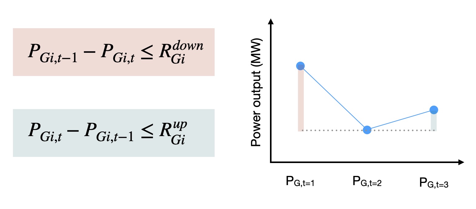
Fig. 5.3 Ramping rate constraints.

5.3.2. Full problem

The full problem we end up with looks like this, with most of the components reflecting 1:1 what we did earlier, except that we add the time (\(t\)) index where necessary:

• 1 Variables: Power output \(P_{Git}\), On/off state of each unit \(u_{it}\)

• 2 Objective (total generation cost, to be minimised): \(C = \sum_{t=1}^T \sum_{i=1}^{n} C_{it} P_{Git}\)

• 3 Constraints:

  • Demand balance constraint: \(\sum_{i=1}^{n} P_{Git} = P_{Dt} \quad \forall t\)

  • Operational constraints for unit \(i\): \(u_{it} P_{Gi}^{min} \leq P_{Git} \leq u_{it} P_{Gi}^{max} \quad \forall i, \forall t\)

  • Ramping constraint: \(P_{Gi, t-1} - P_{Git} \leq R_{Gi}^{down}\) and \(P_{Git} - P_{Gi, t-1} \leq R_{Gi}^{up} \quad \forall i, \forall t\)

  • Binary variable constraint: \(u_{it} \in \{0, 1\} \quad \forall i, \forall t\)

5.4. Power markets

So far we’ve only looked at the generation side, by solving economic dispatch and unit commitment problems. Now we will extend our view slightly to consider the coordination between the producers and consumers of electricity (Fig. 5.4). This means taking a step into power markets. We will focus on modelling a day-ahead wholesale market auction, such as the one operated by EPEX SPOT in Europe.

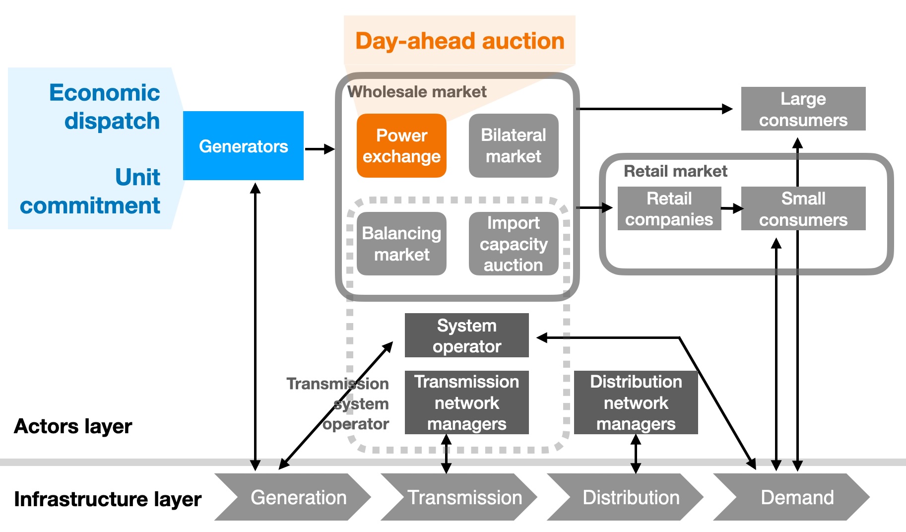
Fig. 5.4 An overarching view of the actors and physical infrastructure in the (Dutch/European) electricity system. Based on a slide by Laurens de Vries. Highlighted in blue is what we have looked at so far: economic dispatch and unit commitment, which takes the perspective of a power plant operator. Now we move on to what is highlighted in orange: the day-ahead auction in the wholesale power market.

In the day-ahead market, electricity generating companies submit generating offers to the pool, while wholesale consumers submit consumption bids. These consumers are for example large industrial entities or companies that sell electricity to retail companies and consumers.

“Blocks” vs “offers and bids”

In the literature, the offers and bids made by participants in the market are generally called “blocks”. To make things easier to follow, here we use “offers” for the generators and “bids” for the demands. Elsewhere, both of these will be called blocks.

A bid for either supply or demand consists of a price and a maximum amount of electricity, e.g. a consumer may be willing to pay a price of 3 EUR/MWh for up to 10 MW of power in the hour of the day for which the auction is taking place.

As market operator, our goal is to maximise social welfare (Fig. 5.5). To do so, we sort the offers from producers by increasing cost, and the bids from consumers by decreasing cost. Consumer surplus is the amount of money that consumers would have been willing to pay but did not have to pay, at the current market price and scheduled demand/supply. Producer surplus is the amount of money that producers receive on top of what they would have been willing to accept. The area between the demand and supply curves represents the social welfare - the sum of producer surplus and consumer surplus.

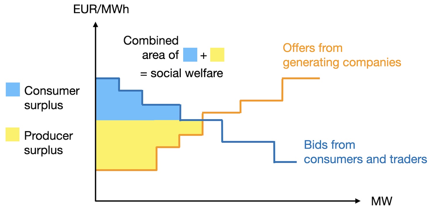
Fig. 5.5 Social welfare as the sum of producer surplus and consumer surplus. Note that since we are considering a single hour, we can consider the scheduled generation or consumption either in terms of MWh (energy) or MW (power), with the same numerical values.

We are looking for both the market price of electricity and the scheduled demand/supply for the hour we are considering (Fig. 5.6). Because we are maximising social welfare, this is the point at which the demand (consumer) and supply (producer) curves meet.

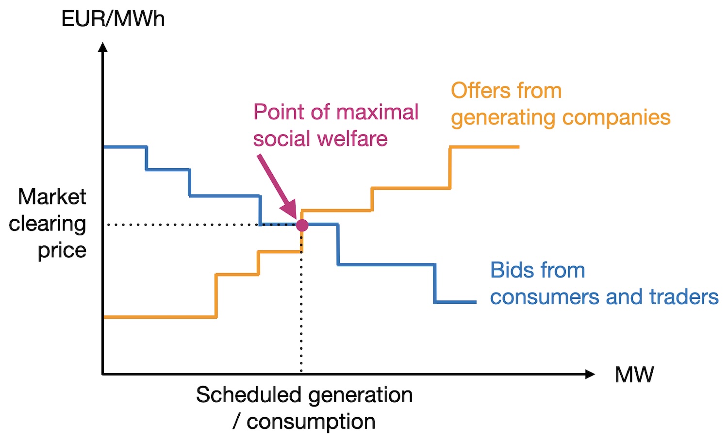
Fig. 5.6 Clearing price and scheduled demand/supply at the point where the supply and demand curves meet.

Clearly, we can implement this procedure in a way that does not require optimisation at all: we can simply look for the point where the two curves meet. But as we will see, if we want to consider aspects like minimum generator outputs, the problem is not so easy to solve any more.

5.5. Modelling a single-period day-ahead market auction

For now, we deal with a simple situation: an auction where we consider just a single time period. This means that we do not yet consider how what happened in the previous hour influences the current hour, or how the current hour affects subsequent hours. In a real market, this may well result in an infeasible solution.

We can formulate the single-period auction as an optimisation problem as follows, with our 2 objective being to maximise social welfare \(SW\):

(5.9)\[\begin{align} \max SW = \sum_{j=1}^{N_D} \sum_{k=1}^{N_{Dj}} \lambda_{Djk} P_{Djk} - \sum_{i=1}^{N_G} \sum_{b=1}^{N_{Gi}} \lambda_{Gib} P_{Gib} \end{align}\]

subject to the following 3 constraints:

(5.10)\[\begin{split}\begin{align} 0 \leq P_{Djk} \leq P^{\max}_{Djk} \ \ \ \forall j,k \\ 0 \leq P_{Gib} \leq P^{\max}_{Gib} \ \ \ \forall i,b \\ \sum_{j=1}^{N_D} \sum_{k=1}^{N_{Dj}} P_{Djk} = \sum_{i=1}^{N_G} \sum_{b=1}^{N_{Gi}} P_{Gib} \end{align}\end{split}\]

with the following parameters and variables:

• 0 Parameters:

  • \(P^{\max}_{Djk}\): the maximum MW size of bid \(k\) asked by consumer \(j\)

  • \(P^{\max}_{Gib}\): the maximum MW size of offer \(b\) offered by generator \(i\)

  • \(\lambda_{Djk}\) : the price (EUR/MWh) of bid \(k\) from consumer \(j\)

  • \(\lambda_{Gib}\) : the price (EUR/MWh) of offer \(b\) from generator \(i\)

• 1 Variables:

  • \(P_{Djk}\) : the power accepted from bid \(k\) by consumer \(j\)

  • \(P_{Gib}\) : the power accepted from offer \(b\) by generator \(i\)

The parameters and variables are indexed as follows:

• \(N_{Dj}\) : the number of bids from consumer \(j\)

• \(N_{Gi}\) : the number of offers from generator \(i\)

• \(N_D\) : the number of consumers

• \(N_G\) : the number of generators

Demand and supply are both variables now

Note that one of the key differences to the economic dispatch and unit commitment problems is that now, demand is not a fixed parameter: it is also in the variables. We, as market operator, need to decide - still under the constraint that demand and supply must be equal to each other - how much of the demand to supply, in a way that optimises social welfare.

5.5.1. Example with three generators and two demands

Source of this example

The example in this section comes from Galiana and Conejo [2018]. You can find more detail there, including an extension of the problem to a multi-period market auction which considers all 24 hours of a day simultaneously.

We consider three generators and two demands. The technical characteristics (generation capacity) of the generating units are:

Unit data	Generator 1	Generator 2	Generator 3
Capacity (MW)	30	25	25

Each generator distributes their possible generation across three offers, while each demand distributes their possible demand across four bids. This makes sense: for example, a large industrial customer might have a strong need for some minimum amount of power to keep machinery running - so they are willing to pay quite a lot for a certain amount of power. And at the other end of the scale, they could produce a bit more in this hour than absolutely necessary - so they are willing to take additional electricity but only if it is not too expensive. These kinds of behaviors are represented in the structure of the bids and offers:

Supply offers	Generator 1			Generator 2			Generator 3
Offer number	1	2	3	1	2	3	1	2	3
Max power \(P^{\max}_{Gib}\) (MW)	5	12	13	8	8	9	10	10	5
Price \(\lambda_{Gib}\) (EUR/MWh)	1	3	3.5	4.5	5	6	8	9	10

Demand bids	Demand 1				Demand 2
Bid number	1	2	3	4	1	2	3	4
Max power \(P^{\max}_{Djk}\) (MW)	8	5	5	3	7	4	4	3
Price \(\lambda_{Djk}\) (EUR/MWh)	20	15	7	4	18	16	11	3

We introduced the parameters, variables, objective function, and constraints above. We will still briefly explain the constraints further.

5.5.1.1. 3 Constraints

There are two types of constraints.

First, the supply offers and demand bids must be within their maximum sizes submitted to the market operator:

(5.11)\[\begin{align} 0 \leq P_{Djk} \leq P_{Djk}^{max} \ \ \ \forall j,k \\ 0 \leq P_{Gib} \leq P_{Gib}^{max} \ \ \ \forall i,b \end{align}\]

Second, the amount of electricity generated must exactly match the demand for electricity - this is a hard requirement, otherwise the power system will collapse. Note that we are making a relatively rough estimation here on the day ahead of the actual operation. On the actual day, other markets will come into play to ensure that generation and demand truly match in each instant.

(5.12)\[\begin{equation} \sum_{j=1}^{N_D} \sum_{k=1}^{N_{Dj}} P_{Djk} = \sum_{i=1}^{N_G} \sum_{b=1}^{N_{Gi}} P_{Gib} \end{equation}\]

5.5.1.2. Solving the auction problem

Once again, we could simply solve this problem graphically by sorting the demand bids and supply offers and looking for the point where the two curves meet (Fig. 5.7).

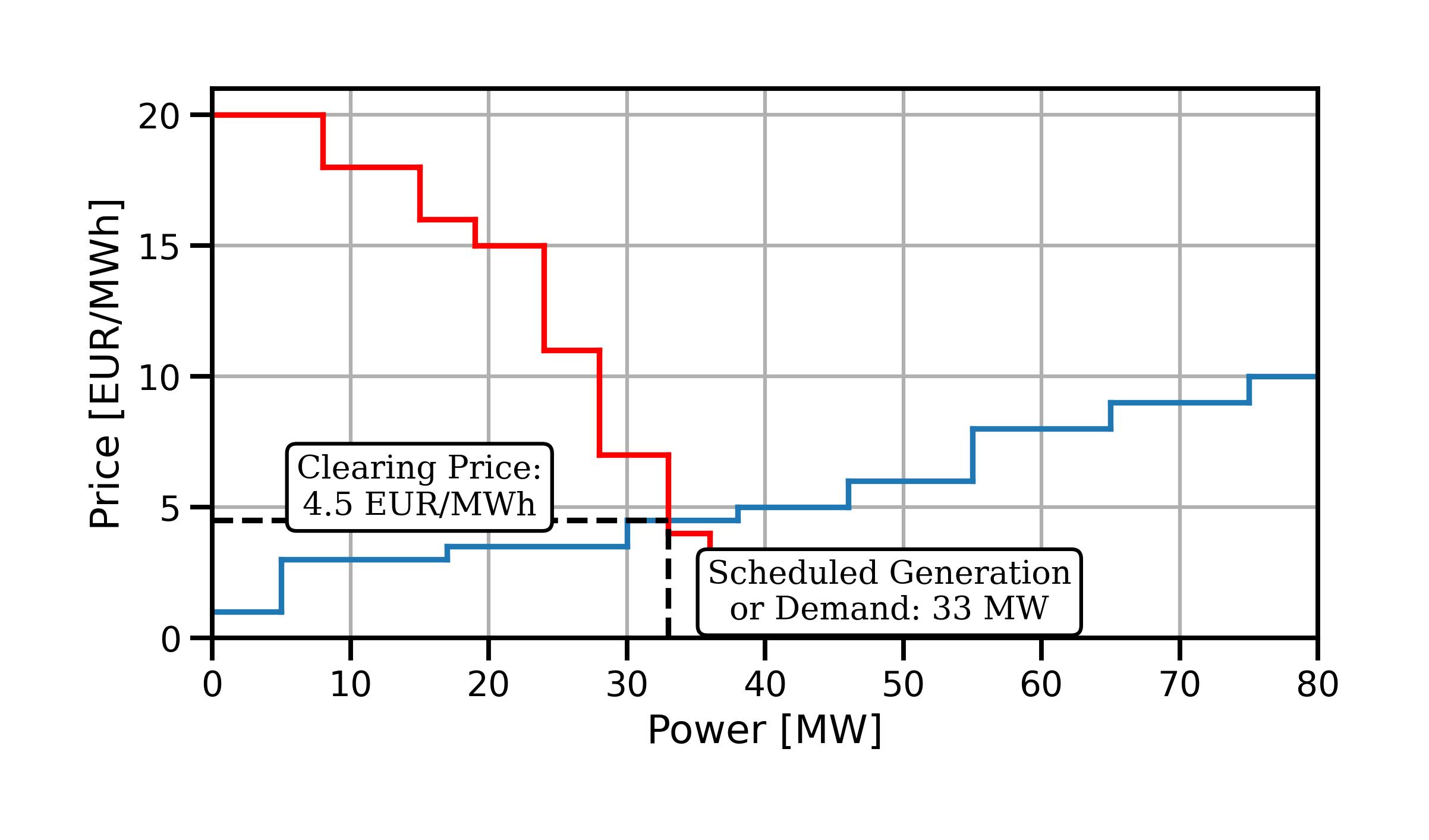
Fig. 5.7 Graphically clearing the power market.

The market-clearing price is 4.5 EUR/MWh, the scheduled generation/demand is 33 MW, and the social welfare is 404 EUR.

If we formulate and solve the optimisation problem from equations (5.9) and (5.10) above with the data from the tables above, we will find exactly these values for the scheduled generation/demand and for the objective function value. But how do we determine the market-clearing price mathematically? When solving this as an optimisation problem, we can use duality here: if only the market-clearing equality constraint (total accepted demand = total accepted generation) is active, then the market-clearing price is equal to the shadow price of that constraint. It represents the marginal cost of electricity.

5.5.2. Considering physical limits through additional constraints

Let’s have a closer look at this solution. We can see that in the optimal solution, all offers from generator 1 are accepted (5 + 12 + 13 = 30 MW, purple in Fig. 5.8), and one bid from generator 2 is partially accepted (3 MW, yellow in the figure).

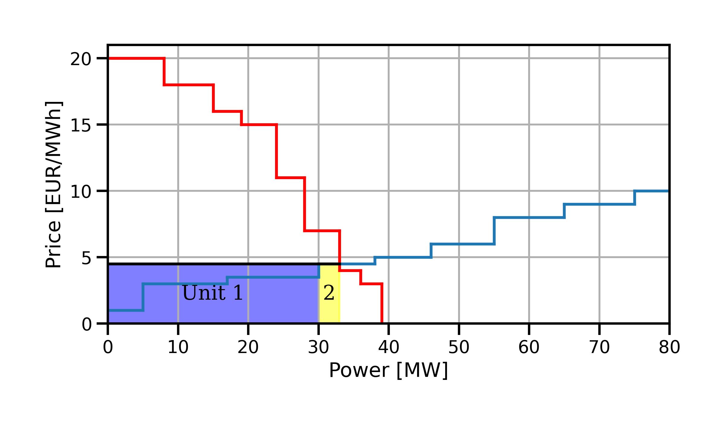
Fig. 5.8 Accepted supply offers in the optimal solution.

In other words, we are asking generator 1 to generate at its maximum output of 30 MW and generator 2 to generate at a mere 3 MW of output.

That’s good news for generator 1. But what if generator 2 has a minimum output below which it cannot operate? Then this solution would not work. We need to extend our problem formulation to consider such physical limits. This is where we bring the additions we made at the beginning of this chapter into our auction problem: additional binary variables to represent on/off state of generators, as well as possible ramping limits on generators.

In our example with three generators, we can consider these additional characteristics of the generators:

Generator Data	Generator 1	Generator 2	Generator 3
Capacity (MW)	30	25	25
Minimum power output (MW)	5	8	10
Ramping up/down limits (MW/h)	5	10	10
Initial power output (MW)	10	15	10

Note that all units are on at the beginning of the period we consider for our auction - their initial power output is non-zero.

This leads to the following additional parameters. Note that because we are considering just a single period (hour), everything that happened in the hour before is fixed - i.e. a parameter for us, not a variable:

• \(P^0_{Gi}\) : the generating level of generator \(i\) just before the auction period

• \(R^{down}_{Gi}\) : the ramping down limit of generator \(i\)

• \(R^{up}_{Gi}\) : the ramping up limit of generator \(i\)

• \(P_{Gi}^{min}\) : the minimum generating level of generator \(i\)

• \(P_{Gi}^{max}\) : the maximum generating level of generator \(i\)

Extending the problem from equations (5.9) and (5.10) above, we end up with the following optimisation problem for our single-period auction. Note that this turns our continuous (LP) problem into a mixed-integer (MILP) one:

• 1 Variables:

  • \(P_{Djk}\) : the power accepted from bid \(k\) by consumer \(j\)

  • \(P_{Gib}\) : the power accepted from offer \(b\) by generator \(i\)

  • \(u_i\): the on/off state of each generator \(i\)

• 2 Objective (like above): \( \max SW = \sum_{j=1}^{N_D} \sum_{k=1}^{N_{Dj}} \lambda_{Djk} P_{Djk} - \sum_{i=1}^{N_G} \sum_{b=1}^{N_{Gi}} \lambda_{Gib} P_{Gib} \)

• 3 Constraints:

  • Maximum demand bid sizes: \(0 \leq P_{Djk} \leq P^{\max}_{Djk} \ \ \ \forall j,k\)

  • Maximum supply offer sizes: \(0 \leq P_{Gib} \leq P^{\max}_{Gib} \ \ \ \forall i,b\)

  • Market clearing constraint: \(\sum_{j=1}^{N_D} \sum_{k=1}^{N_{Dj}} P_{Djk} = \sum_{i=1}^{N_G} \sum_{b=1}^{N_{Gi}} P_{Gib}\)

  • Ramping down constraint: \(P^0_{Gi} - \sum_{b=1}^{N_{Gi}} P_{Gib} \leq R^{down}_{Gi} \ \ \ \forall i\)

  • Ramping up constraint: \(\sum_{b=1}^{N_{Gi}} P_{Gib} - P^0_{Gi} \leq R^{up}_{Gi} \ \ \ \forall i\)

  • Per-generator on/off state and minimum/maximum generation limits: \(u_i P_{Gi}^{\min} \leq \sum_{b=1}^{N_{Gi}} P_{Gib} \leq u_i P_{Gi}^{\max} \ \ \ \forall i\)

Technically speaking, each consumer might also specify that they have a certain minimum demand that must be met no matter how high the power price - in this case we could add a constraint like this:

\(P_{Dj}^{\min} \leq \sum_{k=1}^{N_{Dj}} P_{Djk} \ \ \ \forall j\)

with an associated parameter \(P_{Dj}^{min}\), representing the minimum demand level of demand \(j\).

As minimum demands generally need to be supplied, we would not need to introduce binary variables in the demand constraint: you cannot “turn off” a demand.

5.5.3. Market-clearing price in the MILP formulation

We can solve the above problem easily (or rather, let the computer solve it for us). However, how do we obtain the market-clearing price? In an MILP, we cannot simply use duality to obtain the shadow price. However, we can use a trick:

• First, we solve the MILP problem.

• Then we fix the binary variables to their values from the optimal solution to the MILP problem. We thus turn them from variables into parameters.

• Then we re-solve the resulting continuous (LP) problem. Now we can obtain the shadow price of the market-clearing constraint in the LP problem via the usual route (the dual problem, as solved automatically by the computer) - that will be the market-clearing price.

However, these are the shadow prices of a different problem - a version of the original market auction where we have fixed the binary variables. So this market-clearing price may result in individual generators or consumers making a loss. There are various solutions to this in practice: we can introduce additional constraints, or use the market clearing price from the “trick” above while providing additional out-of-market payments to market participants that are forced to make a loss.

5.6. References

[GC18]

Francisco D. Galiana and Antonio J. Conejo. Economics of Electricity Generation. In Electric Energy Systems. CRC Press, 2nd edition, 2018.

[HL21] (1,2)

Frederick S. Hillier and Gerald J. Lieberman. Introduction to Operations Research. McGraw-Hill Education, New York, NY, 11th edition, 2021. ISBN 9781259872990.