4. Duality and KKT conditions

In this chapter we take a few steps back to consider some of the mathematical properties of the types of problems we are looking at. Understanding these is not strictly necessary - you could just use a modelling language to formulate and let the computer solve your problem while ignoring everything in this chapter.

However, understanding duality and KKT conditions will be useful in various ways. Duality can be exploited to perform sensitivity analyses and is important when using optimisation methods to solve market problems (Section 5). An understanding of KKT conditions will become relevant particularly when we look at mixed complementarity (Section 6) and non-linear programming problems. As you will see below, duality and KKT conditions are also related. Understanding one can help you understand the other, and vice versa.

4.1. Duality

4.1.1. Introduction to duality

In linear programming, for every problem, which we shall call the primal problem, there exists a “mirrored” problem that we call the dual problem. What’s important is that we (or a computer) can follow a set number of rules to transform the primal problem into the dual problem, and having the dual problem available opens up some interesting possibilities. We will get into these rules and the possibilities further below.

What a dual problem is, is best illustrated with an example. Consider this LP problem (from Table 6.1 in [Hillier and Lieberman, 2021]):

(4.1)\[\begin{align} \max &~ Z = 3x_1 + 5x_2 \\ \text{s.t.}&~ x_1 \leq 4 \\ &~ 2x_2 \leq 12 \\ &~ 3x_1 + 2x_2 \leq 18 \\ &~ x_1 \geq 0 \\ &~ x_2 \geq 0 \end{align}\]

The corresponding dual problem is:

(4.2)\[\begin{align} \min &~ W = 4y_1 + 12y_2 + 18y_3 \\ \text{s.t.}&~ y_1 + 3y_3 \geq 3 \\ &~ 2y_2 + 2y_3 \geq 5 \\ &~ y_1 \geq 0 \\ &~ y_2 \geq 0 \\ &~ y_3 \geq 0 \end{align}\]

The color coding in Fig. 4.1 illustrates some important points:

• Green: The dual problem of a maximisation primal problem is a minimisation problem (and vice versa).

• Yellow: Two primal variables lead to two dual constraints. The primal objective function coefficients (3 and 5) are the dual constraint parameters.

• Purple: The “\(\geq 0\)” bounds on the primal variables lead to “\(\geq\)” in the dual constraints.

• Blue: Three primal constraints lead to three dual variables. The primal constraint parameters (4, 12, and 18) are the dual objective function coefficients.

• Cyan: The “\(\leq\)” in the primal constraints leads to “\(\geq 0\)” bounds on the dual variables.

• Red: The coefficients of the dual constraints are a “rotation” of the primal constraint coefficients.

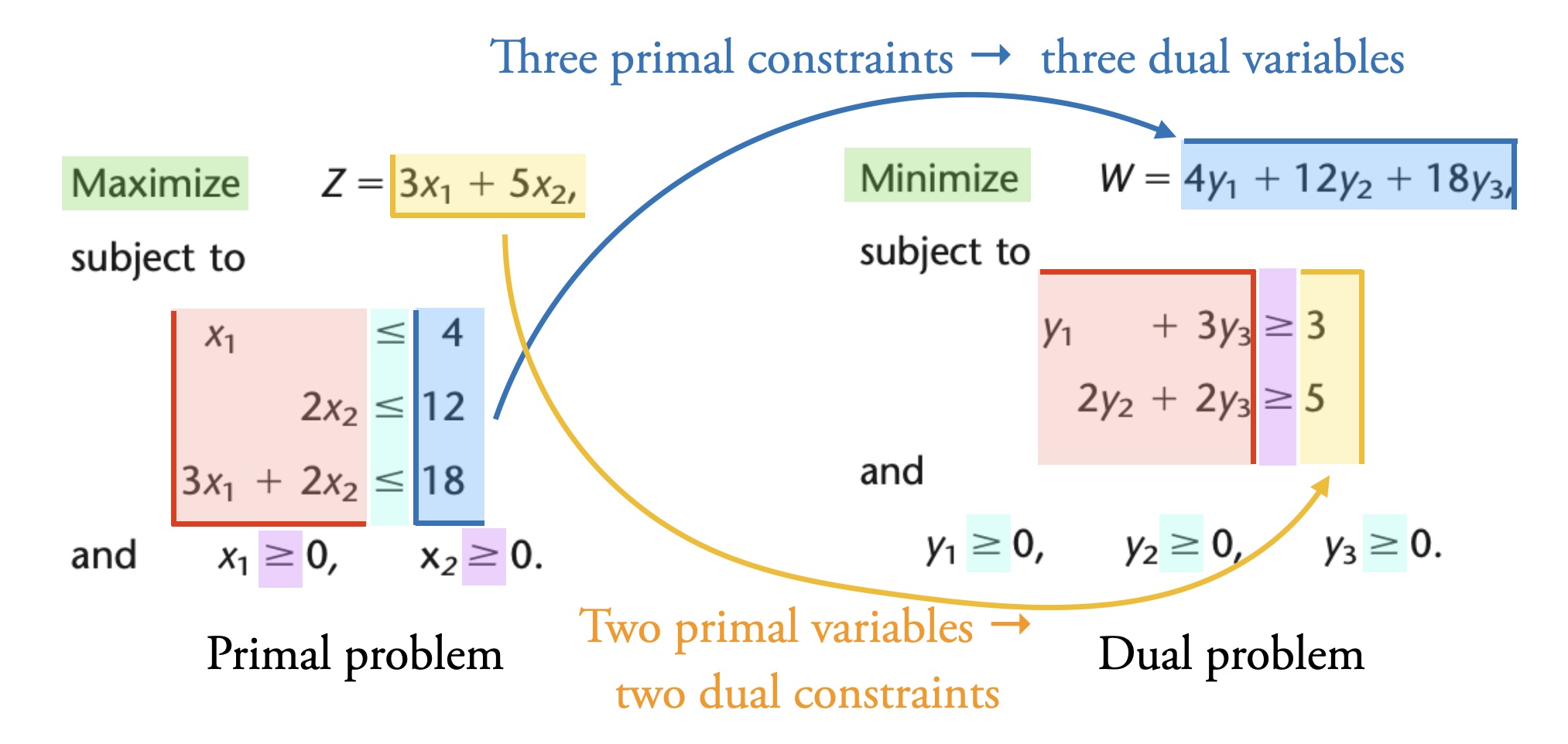
Fig. 4.1 Relationship between primal and dual problem. Adapted from Table 6.1 in [Hillier and Lieberman, 2021].

If we look at the solutions to the primal and dual problems, we see another important property of duality in linear problems: the optimal solution to the primal problem is the same value as the optimal solution to the dual problem. Furthermore, the shadow prices of the primal problem are the optimal variable values of the dual problem, and vice versa. The shadow prices of the primal problem in Fig. 4.1 are \((0, 1.5, 1)\). The value of the variables in the optimal solution to the dual problem are also \((0, 1.5, 1)\).

Strong and weak duality

Weak duality means that the solution to any primal minimisation problem is always greater than or equal to the solution of the corresponding dual (maximisation) problem. Under certain conditions - and this includes the condition that we are dealing with linear optimisation - we also see strong duality, which means that the solution of the primal problem is equal to the solution of the dual problem. We only deal with the linear case here, where strong duality always applies. Thus we will not consider this distinction further, but it is something you will find discussed in detail elsewhere.

4.1.2. Economic dispatch example

We will now revisit the economic dispatch problem from Section 2.1 and formulate the corresponding dual problem. Recall our economic dispatch problem:

(4.3)\[\begin{align} \text{Min.} \; & J = 3P_1 + 4P_2 \\ \text{s.t.} \; & 50 \leq P_1 \leq 300 \\ & 100 \leq P_2 \leq 400 \\ & P_1 + P_2 = 500 \\ \end{align}\]

We also have the variable bounds: \(P_1 \geq 0\) and \(P_2 \geq 0\) (this comes from the physical nature of our system: power plants produce electricity; their power production has to be a positive value).

Now, to make our life easier, we will rewrite this problem into the standard form that we introduced in Section 2.8.1. We separate out the upper and lower limits on generation which are technically separate constraints, and give all the constraints the same sign.

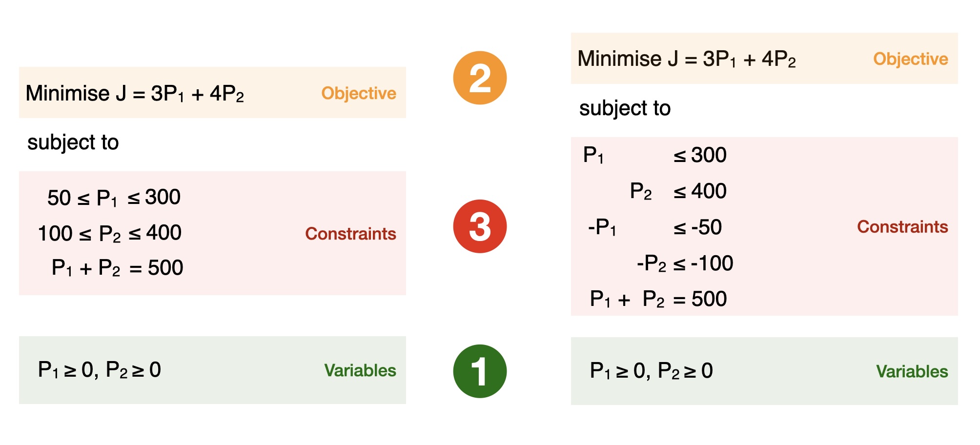
Fig. 4.2 Modifying our economic dispatch example into a standard form.

So our problem now looks like this:

(4.4)\[\begin{align} \text{Min.} \; & J = 3P_1 + 4P_2 \\ \text{s.t.} \; & P_1 \leq 300 \\ & P_2 \leq 400 \\ & -P_1 \leq -50 \\ & -P_2 \leq -100 \\ & P_1 + P_2 = 500 \\ \end{align}\]

It is up to us to pick the naming for the new variables in the dual problem. Often we write down the variable name we’ll use in the dual problem next to the corresponding constraint in the primal problem, which in the above example would look like this:

(4.5)\[\begin{align} \text{Min.} \; & J = 3P_1 + 4P_2 \\ \text{s.t.} \; & P_1 \leq 300 \quad &(X_1) \\ & P_2 \leq 400 \quad &(X_2) \\ & -P_1 \leq -50 \quad &(X_3) \\ & -P_2 \leq -100 \quad &(X_4) \\ & P_1 + P_2 = 500 \quad &(X_5) \\ \end{align}\]

Now, we can use the rules in Table 4.1:

Table 4.1 Conversion from a standard-form minimisation primal problem to its dual problem.

Primal	Dual
Minimise	Maximise
Variables	Constraints
\(\geq 0\)	\(\leq\)
Constraints	Variables
\(=\)	Unconstrained
\(\leq\)	\(\leq 0\)

The dual problem becomes a maximisation problem. There are two primal variables of the form “\(\geq 0\)” so there are two dual constraints of the form “\(\leq\)”. The primal constraints of “\(\leq\)” form become dual variables with bounds “\(\leq 0\)”, while the primal constraint of “\(=\)” form corresponds to a dual variable that is unconstrained or unbounded. We have five primal constraints, which means there are five dual variables.

This is the resulting conversion:

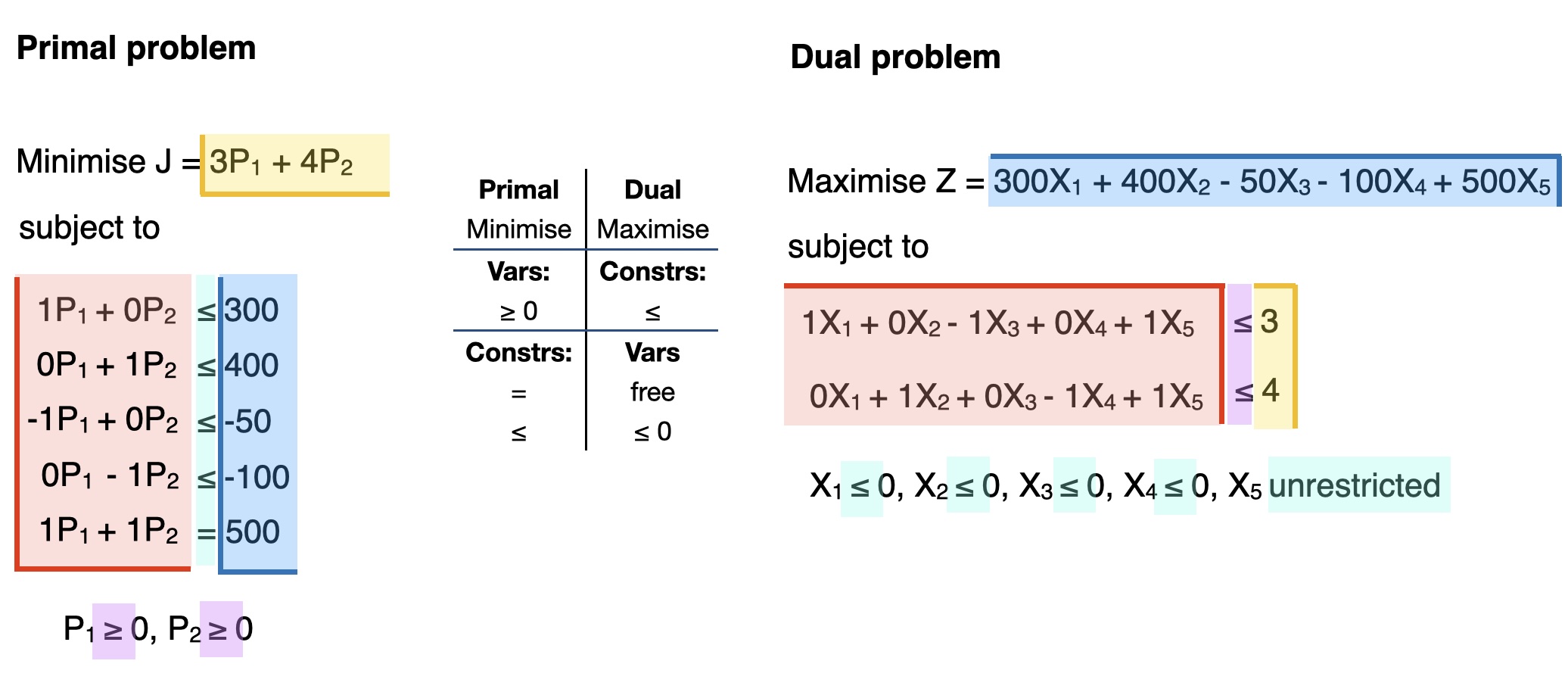
Fig. 4.3 Converting our standard form economic dispatch example into its dual (maximisation) problem.

We end up with this dual problem:

(4.6)\[\begin{align} \text{Max.} \; & Z = 300X_1 + 400X_2 - 50X_3 - 100X_4 + 500X_5 \\ \text{s.t.} \; & X_1 - X_3 + X_5 \leq 3 \\ & X_2 - X_4 + X_5 \leq 4 \\ \end{align}\]

Our new variables are \(X_1 \leq 0, X_2 \leq 0, X_3 \leq 0, X_4 \leq 0\), and \(X_5\) unconstrained. Notice that the objective function coefficients 3 and 4 are the parameters in the dual constraints. Likewise, the primal constraint parameters 300, 400, -50, -100, and 500 are the coefficients in the dual objective function.

Elaboration on constraints (red box in Fig. 4.3)

The left-hand side of the primal and dual constraints can be understood as a rotation of each other. In the context of the economic dispatch example:

• \(P_1\) in the first primal constraint leads to \(X_1\) in the first dual constraint

• \(P_2\) in the second primal constraint leads to \(X_2\) in the second dual constraint

• \(-P_1\) in the third primal constraint leads to \(-X_3\) in the first dual constraint

• \(-P_2\) in the fourth primal constraint leads to \(-X_4\) in the second dual constraint

• \(P_1\) in the fifth primal constraint leads to \(X_5\) in the first dual constraint

• \(P_2\) in the fifth primal constraint leads to \(X_5\) in the second dual constraint

Notice that when there is a factor of \(P_\mathbf{1}\) in a primal constraint, this leads to a term in the first dual constraint. When there is a factor of \(P_\mathbf{2}\), it leads to a term in the second dual constraint. The first primal constraint leads to a factor of \(X_\mathbf{1}\) in the dual constraint, the second primal constraint leads to a factor of \(X_\mathbf{2}\) in the dual constraint, the third primal constraint leads to a factor of \(X_\mathbf{3}\) in the dual constraint, and so on.

We can solve the dual problem to obtain the optimal solution (\(X_1 = -1, X_2 = 0, X_3 = 0, X_4 = 0, X_5 = 4\)). Recall that this solution to the dual problem gives the shadow prices of the primal problem. Looking at the shadow prices also reveals something about the primal constraints. When the shadow price is zero, that means the constraint is non-binding. In our example, only the first constraint (\(P_1 \leq 300\), capacity limit on unit 1) and last constraint (\(P_1 + P_2 = 500\), demand constraint) are active. If the right-hand side of the demand constraint is changed marginally (by one unit) then the optimal value of the objective function will change by \(X_5 = 4\). The objective function value is 1700 in both the primal and dual solution. The optimal value of the objective function in the primal problem is always equal to the optimal value of the dual objective function.

4.1.3. Strategies to convert a primal into its dual problem

The easiest approach to convert a primal problem to its dual problem, and the one we use above, is:

• Rewrite the primal problem to standard form

• Follow the (standard, always same) steps to convert the standard-form problem to its dual

Summary of the recommended approach

Duality: conversion summary in the appendix contains a summary of this recommended approach with a generic example.

You do not have to rewrite to standard form first, however. There is a method called “SOB” which gives you a “map” on how to translate a primal problem into the corresponding dual problem, no matter what exact form it is in. In principle this also always works, but it can be a bit trickier to get your head around and it is easier to make mistakes.

The table in Fig. 4.4 shows you how what the rules in the SOB method are.

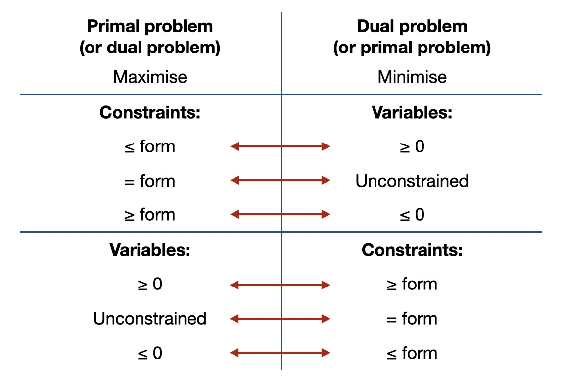
Fig. 4.4 How to convert a primal problem into a dual problem From the “SOB method”: Benjamin (1995), SIAM Review 37(1): 85-87 as summarised in [Hillier and Lieberman, 2021], Table 6.14**

4.1.4. Additional examples

In the appendix chapter “Duality: additional examples” you can find additional examples of duality, including an example of how duality allows you to see the same problem from two perspectives (the buyer and the seller of ingredients for a lunch).

4.2. Karush-Kuhn-Tucker (KKT) conditions

In this section, we introduce the Karush-Kuhn-Tucker (KKT) conditions for convex optimisation problems with equality and inequality constraints. For such convex problems, these conditions form a set of conditions that describe all optimal solutions to the problem at hand. They form the basis for many numerical methods to solve optimisation problems and in simple cases allow determining the solution analytically. They also combine primal and dual variables, which offers additional insight in the solution (e.g., which constraints are active, or what is the electricity price in this system?).

We start from unconstrained optimisation and gradually introduce equality and inequality constraints. We will use an economic dispatch example to illustrate our approach.

4.2.1. Unconstrained optimisation

Let’s go back to basic optimisation (high school mathematics). Whenever you had to optimise (minimise or maximise) a function, you were doing unconstrained optimisation. To determine the maximum or minimum of a certain function, we should take the derivative of that function with respect to (w.r.t.) the decision variable \(x\) and equate it to zero (necessary condition for optimality). Then we take the second order derivative to see if it is a minimum or maximum (sufficient condition). If there are multiple variables, we take partial derivatives.

(4.7)\[\begin{align} \min f(x) & \rightarrow & \frac{\partial f(x)}{\partial x} = 0 \quad \text{(necessary condition)} \\ & & \frac{\partial^2 f(x)}{\partial x^2} > 0 \quad \text{(sufficient condition)} \\ \max f(x) & \rightarrow & \frac{\partial f(x)}{\partial x} = 0 \quad \text{(necessary condition)} \\ & & \frac{\partial^2 f(x)}{\partial x^2} < 0 \quad \text{(sufficient condition)} \\ \end{align}\]

A point that satisfies the necessary condition for optimality (\(\frac{\partial f(x)}{\partial x} = 0\)) is called a stationary point. For convex optimisation problems, we never use the sufficient condition because any stationary point will be a minimum.

4.2.2. Equality constrained optimisation

In energy systems, unfortunately we do not deal with many unconstrained optimisation problems—usually there are at least a few constraints. Consider the example of economic dispatch from Section 2.1. We will again use an economic dispatch example, and build up the complexity of the problem throughout this chapter to illustrate how we can use KKT conditions and duality to solve such problems and interpret their solutions.

Consider two generators \(G_1\) and \(G_2\) with cost structures \(C_1(g_1) = a_1 + b_1 \cdot g_1^2\) and \(C_2(g_2) = a_2 + b_2 \cdot g_2^2\). Note that the cost functions here are quadratic, not linear. This is quite typical in power systems.

Unlike before, we now have a quadratic programming (QP) problem. This is still a convex optimisation problem. Therefore, the techniques we use here also apply to linear programming problems.

Reminder: convex optimisation

Convex optimisation means that we are dealing with convex functions over convex regions. Both linear and quadratic optimisation problems are convex. In general, however, many kinds of non-linear optimisation problems are non-convex, and we cannot apply the techniques we discuss here to them.

We need to dispatch the generators to meet a load \(L\) at minimal cost. We will ignore the capacity constraints of the generators for now. Thus, we have the following optimisation problem:

(4.8)\[\begin{align} & \text{min.} \quad a_1 + b_1 \cdot g_1^2+ a_2 + b_2 \cdot g_2^2 \\ & \text{s.t.} \quad g_1 + g_2 = L \end{align}\]

If we do not consider the equality constraint \(g_1 + g_2 = L\) then the optimal solution to this problem (what minimises operating cost of the system) is \(g_1^* = 0\), \(g_2^*=0\), i.e. not run the generators at all. You can easily confirm this with the necessary condition for optimality: take the derivative of the objective function w.r.t. \(g_1\) and \(g_2\), equate those expressions to zero, and solve for \(g_1\) and \(g_2\). This is the unconstrained optimisation previously discussed.

To deal with the constraint in our optimisation problem, we introduce the Lagrangian. The Lagrangian elevates the constraint to the objective function.

(4.9)\[\begin{equation} \mathcal{L} = (a_1 + b_1 \cdot g_1^2+ a_2 + b_2 \cdot g_2^2) + \lambda \cdot (L - g_1 - g_2) \end{equation}\]

The first part of the Lagrangian is the original objective function. Then we add the constraint multiplied by a Lagrange multiplier \(\lambda\). We want to find an optimal value of \(\lambda\) that coordinates the decision of \(g_1\) and \(g_2\) to ensure that the constraint \(L = g_1^* + g_2^*\) is met at minimum cost.

To do this, we draw on our knowledge of unconstrained optimisation, since now we have a single function, the Lagrangian, to minimise. Thus, we take the first derivative of the Lagrangian w.r.t. \(g_1\) and \(g_2\) and \(\lambda\):

(4.10)\[\begin{align} & \frac{\partial \mathcal{L}}{\partial g_1} = 2 \cdot b_1 \cdot g_1 - \lambda = 0 \\ & \frac{\partial \mathcal{L}}{\partial g_2} = 2 \cdot b_2 \cdot g_2 - \lambda = 0 \\ & \frac{\partial \mathcal{L}}{\partial \lambda} = L - g_1 - g_2 = 0 \end{align}\]

Notice that now we have three equations and three unknowns. So, we can solve for \(g_1\), \(g_2\), and \(\lambda\), which gives the optimal solution to the original optimisation problem. Note that the last equation is identical to our original constraint. A solution to the system of equations above will hence be as such that \(g_1\) and \(g_2\) jointly meet the load \(L\).

Now we will generalise the Lagrangian to any equality constrained optimisation problem. Consider the following minimisation problem with equality constraints \(h_i(x)\):

(4.11)\[\begin{align} \text{min.} \; & f(x) \\ \text{s.t.} \; & h_i(x) = 0 \quad (\lambda_i) \quad \forall i \in \{1,2,...,m\} \end{align}\]

The equality constraints are written in standard form (as introduced in Section 2.8.1), so we have “= 0” on the right-hand side. There are \(m\) equality constraints. We associate a Lagrange multiplier \(\lambda_i\) to each constraint.

The Lagrangian is then:

(4.12)\[\begin{equation} \mathcal{L} = f(x) + \sum_{i=1}^m \lambda_i \cdot h_i(x) \end{equation}\]

We can find the optimal solution (\(x^*, \lambda_i^*\)) to the original optimisation problem by taking the derivative of the Lagrangian w.r.t. the decision variables \(x\) and w.r.t. the Lagrange multipliers \(\lambda_i\). Notice that taking \(\frac{\partial \mathcal{L}}{\partial \lambda_i} = 0\) recovers the equality constraints \(h_i(x) = 0\).

(4.13)\[\begin{align} & \frac{\partial \mathcal{L}}{\partial x} = 0 \\ & \frac{\partial \mathcal{L}}{\partial \lambda_i} = h_i(x) = 0 \quad \forall i \in \{1,2,...,m\} \end{align}\]

Notation and standard form

You will notice that in this section, we write all constraints in a standard form with zeros on the right-hand side (i.e., \(=0\) or \(\leq 0\) for equality constraints below). This ensures that you don’t make mistakes when you’re constructing the Lagrangian. In Section 4.1 above we used a different standard form that makes it easier to construct the dual problem. This highlights that there is no generally “correct” approach to write a standard form. It makes sense to go with an approach that works best for what you are doing.

The equality constrained optmisation problem also has a graphical interpretation. Fig. 4.5 shows the graphical interpretation of our economic dispatch example.

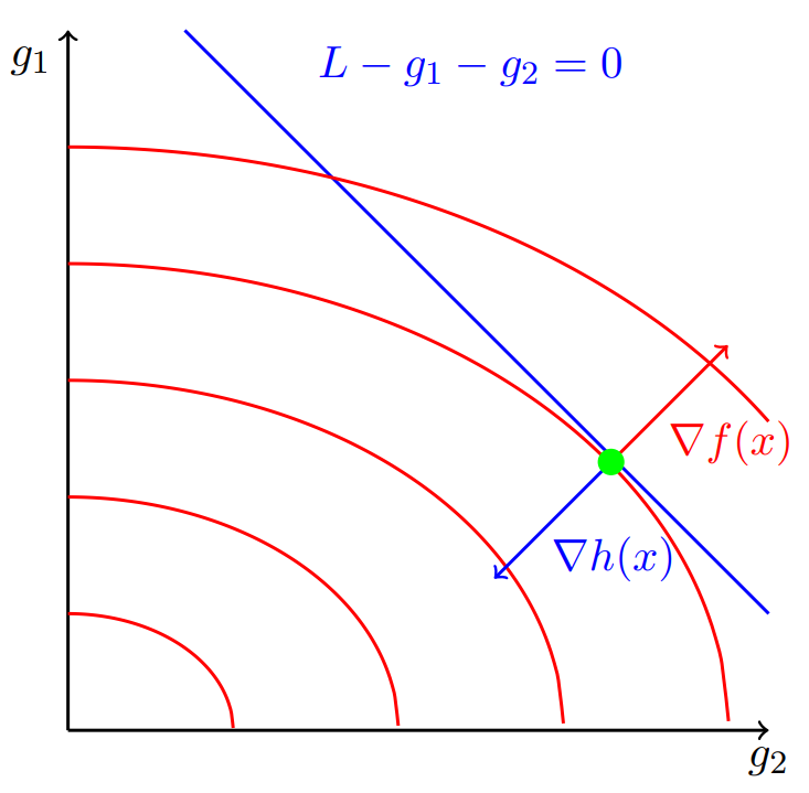
Fig. 4.5 Graphical representation of the equality constrained economic dispatch problem

\(g_1\) and \(g_2\) are on the axes. The red contour lines are constant values of the objective function (total operating cost). The total operating cost increases as \(g_1\) and \(g_2\) increase. The blue line is the equality constraint. The green dot is the optimal solution. At this point, the gradient of the objective function \(\nabla f(x)\) (red arrow) is (1) perpendicular to the constraint and (2) parallel to the gradient of the constraint \(\nabla h(x)\) (blue arrow). This can be expressed as:

(4.14)\[\begin{equation} \nabla f(x) + \lambda \cdot \nabla h(x) = 0 \end{equation}\]

4.2.3. Inequality and equality constrained optimisation

In energy systems, we not only have equality constraints, but also inequality constraints. For example, returning to the economic dispatch example, the generators have maximum generation capacity constraints \(\overline{G_1}\) and \(\overline{G_2}\) and cannot run at negative output (lower bound of zero). The optimisation problem becomes:

(4.15)\[\begin{align} \text{min.} \; & a_1 + b_1 \cdot g_1^2+ a_2 + b_2 \cdot g_2^2 \\ \text{s.t.} \; & g_1 + g_2 = L \\ & 0 \leq g_1 \leq \overline{G_1} \\ & 0 \leq g_2 \leq \overline{G_2} \end{align}\]

To solve the problem with equality and inequality constraints, we extend our graphical interpretation. The grey area in Fig. 4.6 is the feasible region because it represents the feasible range of output of \(g_1\) and \(g_2\). The set of feasible solutions—the values of \(g_1\) and \(g_2\) that satisfy both the equality and inequality constraints—lie on the blue line within the grey area. This is exactly what we already did in Section 2.1, just with different notation for our generation and demand constraints - and as will become clear in FIGURE, a key difference in where the optimal solution lies, since we are dealing with a quadratic rather than a linear problem.

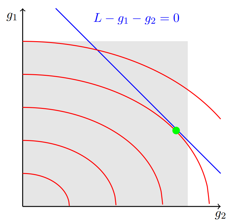
Fig. 4.6 Graphical representation of the equality and inequality constrained economic dispatch problem

The optimal solution needs to be part of the feasible solution set. In this case, we see that the optimal solution (green dot) is indeed in the feasible area. Thus the inequality constraints \(0 \leq g_1 \leq \overline{G_1}\) and \(0 \leq g_2 \leq \overline{G_2}\) actually do not play a role in this particular example.

From linear to quadratic problems

Recall that in Section 2.1, we were able to say that an optimal solution (if it exists) would always lie at one of the corners of the feasible region. Here, however, we now have a solution in the interior of the feasible region. You can see why when you look at the contour lines: they are no longer linear. We are dealing with a quadratic problem here.

However, it will not always be the case that none of the inequality constraints play a role. What if the capacity limits on \(g_1\) and \(g_2\) do play a role? Then we want to figure out which inequality constraints are active. If we can identify the active constraints, we can replace these constraints with equality constraints (e.g., \(g_1 \leq \overline{G_1}\) becomes \(g_1 = \overline{G_1}\)) and ignore all inactive constraints (because they don’t influence the solution). Then we are left with an equality constrained optimisation problem which we know how to solve.

For most problems, we do not know which constraints will be active/binding. Luckily, we can use a set of optimality conditions called Karush-Kuhn-Tucker (KKT) conditions to reflect the fact that in some cases inequality constraints are binding and in some cases they are not.

Consider the general inequality and equality constrained optimisation problem written in standard form:

(4.16)\[\begin{align} \text{min.} \; & f(x) \\ \text{s.t.} \; & h_i(x) = 0 \quad (\lambda_i) \quad \forall i \in \{1,2,...,m\} \\ & g_j(x) \leq 0 \quad (\mu_j) \quad \forall j \in \{1,2,...,n\} \end{align}\]

There are \(m\) equality constraints associated with Lagrange multipliers \(\lambda_i\) and \(n\) inequality constraints associated with Lagrange multipliers \(\mu_j\).

The Lagrangian is:

(4.17)\[\begin{equation} \mathcal{L} = f(x) + \sum_{i=1}^m \lambda_i \cdot h_i(x) + \sum_{j=1}^{n} \mu_j \cdot g_j(x) \end{equation}\]

To formulate the Lagrangian, we followed the same logic as before: elevate the equality and inequality constraints to the Lagrangian. The Lagrangian has three components: the original objective function, the equality constraints multiplied by their Lagrange multipliers, and the inequality constraints multiplied by their Lagrange multipliers.

Then, with the help of the Lagrangian, we derive the following set of equations that characterises the optimal solution. These are the KKT conditions.

(4.18)\[\begin{split}\begin{align} & \frac{\partial \mathcal{L}}{\partial x} = 0 \quad & (\text{Optimality conditions})\\ & \frac{\partial \mathcal{L}}{\partial \lambda_i} = h_i(x) = 0 \quad \forall i \in \{1,2,...,m\} \quad & (\text{Primal feasibility}) \\ & \frac{\partial \mathcal{L}}{\partial \mu_j} = g_j(x) \leq 0 \quad \forall j \in \{1,2,...,n\} \quad & (\text{Primal feasibility}) \\ & \mu_j \cdot g_j(x) = 0 \quad \forall j \in \{1,2,...,n\} \quad & (\text{Complementary slackness conditions}) \\ & \mu_j \geq 0 \quad \forall j \in \{1,2,...,n\} & (\text{Dual feasibility}) \end{align}\end{split}\]

Note on inequality signs in standard form

• Note that all constraints in a standard form have zeros on the right-hand side (i.e., \(=0\) or \(\leq 0\) for equality constraints below).

• Inequality constraints are always of the form \(g_j(x) \leq 0\), not \(g_j(x) \geq 0\). Only if you write all inequality constraints as \(g_j(x) \leq 0\), the signs of the Lagrangian above are correct!

Let’s look at each of these equations in a little more detail. We have:

1. Derivative of Lagrangian w.r.t. decision variables \(x\) equal to zero \(\rightarrow\) optimality conditions

2. Derivative of Lagrangian w.r.t. Lagrange multipliers \(\lambda_i\) (equality constraints) \(\rightarrow\) primal feasibility (solution is feasible with respect to the primal constraints)

3. Derivative of Lagrangian w.r.t. Lagrange multipliers \(\mu_j\) (inequality constraints) \(\rightarrow\) primal feasibility

4. The multiplication of a Lagrange multiplier with its associated inequality constraint is zero \(\rightarrow\) complementary slackness conditions (indicates that in some cases the inequality constraints might not be binding)

5. Lagrange multipliers \(\mu_j\) need to be positive or zero \(\rightarrow\) dual feasibility

Let’s look more carefully at the interpretation of the complementary slackness conditions—the last two constraints in Equation (4.18):

(4.19)\[\begin{align} & \mu_j \cdot g_j(x) = 0 \quad \forall j \in \{1,2,...,n\} \\ & \mu_j \geq 0 \quad \forall j \in \{1,2,...,n\} \end{align}\]

If a constraint is binding, we can replace the inequality sign with an equality sign, so we have \(g_j(x) = 0\). Then, the Lagrange multiplier \(\mu_j\) may take on any non-zero value (\(\mu_j \geq 0\)). Since \(g_j(x) = 0\) in this case, the constraint \(\mu_j \cdot g_j(x) = 0\) will be satisfied no matter the value of \(\mu_j\). On the other hand, if the constraint is non-binding (\(g_j(x) < 0\)), the Lagrange multiplier will equal zero (\(\mu_j = 0\)). Otherwise the constraint \(\mu_j \cdot g_j(x) = 0\) would be violated. This shows that an inequality constraint can only affect the optimal solution if it is binding. Note that these constraints are non-linear.

Now we want to find a solution to the set of equations (values for \(x\), \(\lambda_i\), and \(\mu_j\)). For most, but not all, convex problems, these conditions are sufficient and necessary conditions for optimality, so the obtained solution would be an optimal solution (note once again, that KKT conditions can only be formulated for convex problems - this includes the kinds of problems we discuss here, purely linear problems and problems with a quadratic (nonlinear) objective function).

Condensed form of KKT conditions

Note that sometimes KKT conditions are written in condensed form:

(4.20)\[\begin{align} & \nabla f(x) + \sum_{i=1}^m \lambda_i \cdot \nabla h_i(x) + \sum_{j=1}^{n} \mu_j \cdot \nabla g_j(x) = 0 \\ & \mu_j \cdot g_j(x) = 0 \quad \forall j \in \{1,2,...,n\} \\ & \mu_j \geq 0 \quad \forall j \in \{1,2,...,n\} \end{align}\]

Let’s revisit the economic dispatch example and apply KKT conditions. In the standard form we want to use here, the constraints are written separately with a zero on the right-hand sign and “=” or “\(\leq\)” signs:

(4.21)\[\begin{align} \text{min.} \; & a_1 + b_1 \cdot g_1^2+ a_2 + b_2 \cdot g_2^2 & \\ \text{s.t.} \; & g_1 + g_2 - L = 0 \quad &(\lambda) \\ & - g_1 \leq 0 \quad &(\mu_1) \\ & g_1 - \overline{G_1} \leq 0 \quad &(\mu_2) \\ & - g_2 \leq 0 \quad &(\mu_3) \\ & g_2 - \overline{G_2} \leq 0 \quad &(\mu_4) \end{align}\]

This makes it easy to write the Lagrangian, following Equation (4.17):

(4.22)\[\begin{align} \mathcal{L} = & a_1 + b_1 \cdot g_1^2+ a_2 + b_2 \cdot g_2^2 + \lambda \cdot ( g_1 + g_2 - L ) \\ & + \mu_1 \cdot ( - g_1) + \mu_2 \cdot ( g_1 - \overline{G_1}) \\ & + \mu_3 \cdot ( - g_2 ) + \mu_4 \cdot ( g_2 - \overline{G_2}) \end{align}\]

Then we derive the KKT conditions:

(4.23)\[\begin{align} & \frac{\partial \mathcal{L}}{\partial g_1} = 2 \cdot b_1 \cdot g_1 + \lambda - \mu_1 + \mu_2 = 0 \quad & (\text{Optimality conditions}) \\ & \frac{\partial \mathcal{L}}{\partial g_2} = 2 \cdot b_2 \cdot g_2 + \lambda - \mu_3 + \mu_4 = 0 \quad & (\text{Optimality conditions}) \\ & \frac{\partial \mathcal{L}}{\partial \lambda} = g_1 + g_2 - L = 0 \quad & (\text{Primal feasibility (equality constraint)}) \\ & - g_1 \leq 0 \quad & (\text{Primal feasibility (inequality constraint}) \\ & g_1 - \overline{G_1} \leq 0 \quad & (\text{Primal feasibility (inequality constraint}) \\ & - g_2 \leq 0 \quad & (\text{Primal feasibility (inequality constraint}) \\ & g_2 - \overline{G_2} \quad & (\text{Primal feasibility (inequality constraint}) \\ & \mu_1 \cdot ( - g_1) = 0 \quad & (\text{Complementary slackness conditions}) \\ & \mu_2 \cdot ( g_1 - \overline{G_1}) = 0 \quad & (\text{Complementary slackness conditions}) \\ & \mu_3 \cdot ( - g_2 ) = 0 \quad & (\text{Complementary slackness conditions}) \\ & \mu_4 \cdot ( g_2 - \overline{G_2}) = 0 \quad & (\text{Complementary slackness conditions}) \\ & \mu_1, \mu_2, \mu_3, \mu_4 \geq 0 \quad & (\text{Dual feasibility}) \end{align}\]

Clearly, this is a large set of equations. This problem is not trivial to solve because the complementary slackness constraints are non-linear. For simple cases addressed in this course, we can solve the problem by using trial-and-error: “What if a certain constraint \(g_j(x)\) is binding? Does that lead to a feasible solution? Is the solution optimal?” In this example, there are four inequality constraints so in theory there are 16 (\(=2^4\)) possible combinations. However, some combinations are not possible, for example if \(g_1 = 0\), then \(g_1 \neq \overline{G_1}\). By trying different combinations of constraints, we come up with candidate solutions, then assess whether they are optimal or not.

Let’s look at the problem graphically (see Fig. 4.7). We assume that the feasible range of values for \(g_2\) reduces so the original optimal solution (green dot) is no longer in the feasible set. By looking at the graph and reasoning, we can suppose that the upper capacity limit of \(g_2\) will be binding. So, we will test the solution in which \(g_1\) is producing somewhere in its operating range \(0 < g_1 < \overline{G_1}\) (the inequality constraints are non-binding) and \(g_2\) is operating at maximum capacity \(g_2 = \overline{G_2}\). The solution still needs to satisfy the equality constraint (be on the blue line).

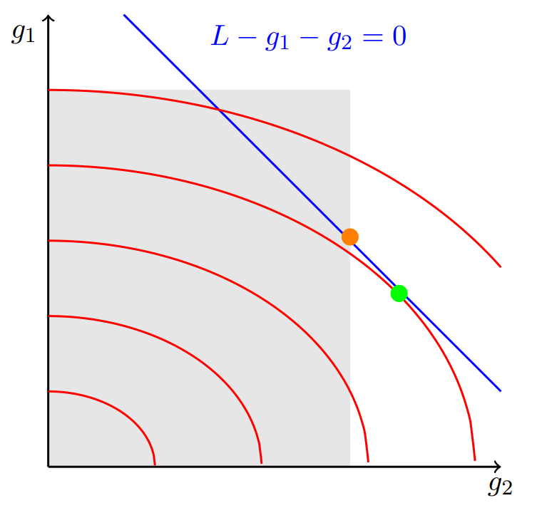
Fig. 4.7 Graphical representation of the economic dispatch problem with reduced feasible range for \(g_2\)

Given this test solution, we know that \(\mu_1\), \(\mu_2\), \(\mu_3\) \(= 0\) and \(\mu_4 \neq 0\). This simplifies the set of KKT conditions to:

(4.24)\[\begin{align} & \frac{\partial \mathcal{L}}{\partial g_1} = 2 \cdot b_1 \cdot g_1 + \lambda = 0 \\ & \frac{\partial \mathcal{L}}{\partial g_2} = 2 \cdot b_2 \cdot g_2 + \lambda + \mu_4 = 0 \\ & \frac{\partial \mathcal{L}}{\partial \lambda} = g_1 + g_2 - L = 0 \\ & - g_1 < 0 \\ & g_1 - \overline{G_1} < 0 \\ & g_2 = \overline{G_2} \\ & \mu_1, \mu_2, \mu_3 = 0 \\ & \mu_4 \geq 0 \end{align}\]

The only unknown variables are \(g_1\), \(\lambda\), and \(\mu_4\), which we can solve for. If we can find a solution, it is optimal. We can also ask ourselves “Does the solution make sense? Is there an alternative set of binding inequality constraints that would yield a better solution?” to check that indeed we have found the optimal solution. The new solution—orange dot in Fig. 4.7—satisfies the constraints but comes at a higher total operating cost than before.

Ok, you might ask: what is this all good for? KKT conditions can help us find the optimal solutions to nonlinear problems (we don’t need them for linear problems), and we will apply them when looking at mixed complementarity problems in Section 6. But they also give us a different view on duality, and this is what we want to turn our attention to last.

4.3. The connection between duality and KKT conditions

We know that for every primal problem, there exists a dual problem, but how do we formulate the dual problem?

Recall the general formulation of a primal problem:

(4.25)\[\begin{align} \text{min.} \; & f(x) \\ \text{s.t.} \; & h_i(x) = 0 \quad (\lambda_i) \quad \forall i \in \{1,2,...,m\} \\ & g_j(x) \leq 0 \quad (\mu_j) \quad \forall j \in \{1,2,...,n\} \end{align}\]

The Lagrangian is:

(4.26)\[\begin{equation} \mathcal{L}(x,\lambda,\mu) = f(x) + \sum_{i=1}^m \lambda_i \cdot h_i(x) + \sum_{j=1}^{n} \mu_j \cdot g_j(x) \end{equation}\]

The Lagrangian dual function, or dual function, is the minimum of the Lagrangian:

(4.27)\[\begin{equation} \mathcal{D}(\lambda,\mu) = \text{inf}_{x} \{\mathcal{L}(x,\lambda,\mu)\} = \text{inf}_{x} \{ f(x) + \sum_{i=1}^m \lambda_i \cdot h_i(x) + \sum_{j=1}^{n} \mu_j \cdot g_j(x) \} \end{equation}\]

with “inf” a generalisation of the “min” operator.

The dual function defines a lower bound on the optimal value \(p^*\) of the primal problem: \(\mathcal{D}(\lambda,\mu) \leq p^*\) for any \(\mu \geq 0\) and any \(\lambda\). We want to find the best possible lower bound of the primal problem, which means maximising the lower bound:

(4.28)\[\begin{split}\begin{align} \text{max.} \; & \mathcal{D}(\lambda,\mu) \\ \text{s.t.} \; & \mu_j \geq 0 \quad \forall j \in \{1,2,...,n\} \end{align}\end{split}\]

This is the dual problem. We denote the optimal value of this problem as \(d^*\).

As mentioned at the beginning, strong duality is when the optimal value of the primal equals the optimal value of the dual. In our new terminology, this is written as \(d^* = p^*\). Strong duality can be used to show that a solution that satisfies the KKT conditions must be an optimal solution to the primal and dual problems. In other words, the KKT conditions are necessary and sufficient conditions for optimality.

Weak duality is when \(d^* \leq p^*\). This holds even for non-convex problems. In such problems, \(p^* - d^*\) is referred to as the duality gap.

In practice, we do not need to start from the general expression in Equation (4.28) to derive the dual problem. Instead, we can simply follow the steps introduced above (Section 4.1.3): write the primal problem in standard form and then mechanistically translate it into its dual counterpart.

4.4. Further reading

For more background on duality and to dive deeper into the mathematics, we suggest reading Chapter 5 of Boyd and Vandenberghe [2004] which is freely available online.

For alternative introductions to duality and KKT conditions based on a vector/matrix formulation, see Appendix B in Morales et al. [2014] (possibly available for free as an ebook if you are connected to a university network).

4.5. References

[BV04]

Stephen Boyd and Lieven Vandenberghe. Convex Optimization. Cambridge University Press, Cambridge, UK ; New York, 1st edition edition, March 2004. ISBN 978-0-521-83378-3.

[HL21] (1,2,3)

Frederick S. Hillier and Gerald J. Lieberman. Introduction to Operations Research. McGraw-Hill Education, New York, NY, 11th edition, 2021. ISBN 9781259872990.

[MCM+14]

Juan M. Morales, Antonio J. Conejo, Henrik Madsen, Pierre Pinson, and Marco Zugno. Integrating Renewables in Electricity Markets: Operational Problems. Volume 205 of International Series in Operations Research & Management Science. Springer US, Boston, MA, 2014. ISBN 978-1-4614-9410-2 978-1-4614-9411-9. doi:10.1007/978-1-4614-9411-9.